Kalman filter Kalman Filter Kalman filter is used to filter true - PowerPoint PPT Presentation

Kalman filter

Kalman Filter Kalman filter is used to filter “true” system states from noisy measurements T o apply the filter, we have to have good model of a system Common use cases: localization of robots, spaceships, ... radar tracking ...

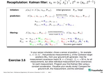
Model System state x k = F k x k − 1 + B k u k + w k Observations z k = H k x k + v k Errors w k ∼ N (0 , Q k ) v k ∼ N (0 , R k )

Kalman filter Kalman filter is represented by two variables at any time k the estimate of state at time k given ˆ x k | k allthe observations until and including time k error covariance matrix showing the P k | k precision of state estimates

Filtering steps Prediction Based on previous state we predict the next state and variation of the system Update Based on the observation we correct the system state and covariance estimates

Predict The state and covariance are predicted from model x k | k − 1 = F k ˆ x k − 1 | k − 1 + B k − 1 u k − 1 ˆ P k | k − 1 = F k P k − 1 | k − 1 F T k + Q k − 1

Update The state is updated as x k | k = ˆ ˆ x k | k − 1 + K k ( z k − H k ˆ x k | k − 1 ) where is called the Kalman gain K k The estimate covariance is P k | k = ( I − K k H k ) P k | k − 1

Kalman gain Kalman gain gives an optimal weight for including the observation information It minimizes the mean square error criteria x k | k | 2 ] . E[ | x k − ˆ Which means we are minimizing tr ( P k | k )

Deriving the Kalman gain Using the model terms it is easy to show x k | k ) = ( I − K k H k ) P k | k − 1 ( I − K k H k ) T + K k R k K T P k | k = cov( x k − ˆ k Expanding it, we get P k | k = P k | k − 1 − K k H k P k | k − 1 − P k | k − 1 H T k K T k + K k ( H k P k | k − 1 H T k + R k ) K T k = P k | k − 1 − K k H k P k | k − 1 − P k | k − 1 H T k K T k + K k S k K T k Setting the derivative to zero yields ∂ tr( P k | k ) = − 2( H k P k | k − 1 ) T + 2 K k S k = 0 ∂ K k K k = P k | k − 1 H T k S − 1 k

Extended Kalman filter Say we have a nonlinear model x k = f ( x k − 1 , u k ) + w k z k = h ( x k ) + v k Kalman filter cannot be applied directly However, we can linearize the model at each step and use it in the model

-0.2 -0.2 -0.3 Voltage -0.3 Voltage -0.4 -0.4 -0.5 -0.5 50 10 20 30 40 50 10 20 30 40 Figure 4.6: Second simulation: = 1 . The filter is slower to re- R Figure 4.7: Third simulation: = 0.0001 . The filter responds to R spond to the measurements, resulting in reduced estimate variance. measurements quickly, increasing the estimate variance. Parameter influence