Kalman Filtering Notes Portions of these notes are adapted from [3], - PDF document

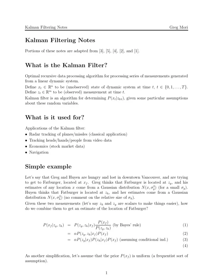
Kalman Filtering Notes Greg Mori Kalman Filtering Notes Portions of these notes are adapted from [3], [5], [4], [2], and [1]. What is the Kalman Filter? Optimal recursive data processing algorithm for processing series of measurements generated from a linear dynamic system. Define x t ∈ R n to be (unobserved) state of dynamic system at time t , t ∈ { 0 , 1 , . . ., T } . Define z t ∈ R m to be (observed) measurement at time t . Kalman filter is an algorithm for determining P ( x t | z 0: t ), given some particular assumptions about these random variables. What is it used for? Applications of the Kalman filter: • Radar tracking of planes/missles (classical application) • Tracking heads/hands/people from video data • Economics (stock market data) • Navigation Simple example Let’s say that Greg and Huyen are hungry and lost in downtown Vancouver, and are trying to get to Fatburger, located at x f . Greg thinks that Fatburger is located at z g , and his estimates of any location x come from a Gaussian distribution N ( x, σ 2 g ) (for a small σ g ). Huyen thinks that Fatburger is located at z h , and her estimates come from a Gaussian distribution N ( x, σ 2 h ) (no comment on the relative size of σ h ). Given these two measurements (let’s say z h and z g are scalars to make things easier), how do we combine them to get an estimate of the location of Fatburger? P ( z g , z h | x f ) P ( x f ) P ( x f | z g , z h ) = P ( z g , z h ) (by Bayes’ rule) (1) = αP ( z g , z h | x f ) P ( x f ) (2) = αP ( z g | x f ) P ( z h | x f ) P ( x f ) (assuming conditional ind.) (3) (4) As another simplification, let’s assume that the prior P ( x f ) is uniform (a frequentist sort of assumption). 1

Kalman Filtering Notes Greg Mori Then, P ( x f | z g , z h ) ∝ P ( z g | x f ) P ( z h | x f ) (5) � � � � − 1 − 1 2( z g − x f ) 2 /σ 2 2( z h − x f ) 2 /σ 2 ∝ exp exp (6) g h ( z g − x f ) 2 σ 2 h + ( z h − x f ) 2 σ 2 � � − 1 g = exp (7) σ 2 2 h σ 2 g ( σ 2 h + σ 2 g ) x 2 f − 2( z g σ 2 h + z h σ 2 g ) x f + ( z 2 g σ 2 h + z 2 h σ 2 g ) � − 1 � = exp (8) σ 2 h σ 2 2 g ( σ 2 h + σ 2 g ) x 2 f − 2( z g σ 2 h + z h σ 2 � g ) x f � − 1 ∝ exp (9) σ 2 2 h σ 2 g This looks messy, but can be converted into something familiar, using the trick of “completing the square.” 2 a ) 2 + ( c − b 2 ax 2 + bx + c = a ( x − − b 4 a ) (10) Applying this trick to Equation 9 gives us: � � 2 � � σ 2 g + σ 2 x f − 2 z g σ 2 h + 2 z h σ 2 − 1 � � h g P ( x f | z g , z h ) ∝ exp + R (11) g σ 2 2( σ 2 2 σ 2 h + σ 2 g ) h   � 2 � z g σ 2 h + z h σ 2 x f − g  − 1 ( σ 2  h + σ 2 g )  ∝ exp (12)   � 2 2  �  σ h σ g √  σ 2 g + σ 2 h z g σ 2 h + z h σ 2 σ 2 h σ 2 i.e. a Gaussian distribution with mean g and variance g ( σ 2 h + σ 2 g ) σ 2 g + σ 2 h More General Assumptions We will make the following assumptions: • Markovian conditional independence for states, P ( x t | x 0: t − 1 ) = P ( x t | x t − 1 ), and measure- ments P ( z t | x 0: t , z 0: t − 1 ) = P ( z t | x t ) • x 0 is drawn from a Gaussian distribution N ( µ 0 , Σ 0 ) • P ( x t | x t − 1 ) is a linear Gaussian distribution, P ( x t | x t − 1 ) = N ( Ax t − 1 , Σ x ). I.e. x t = Ax t − 1 + w t , linear transformation of x t − 1 plus (white) Gaussian noise. • P ( z t | x t ) is a linear Gaussian distribution, P ( z t | x t ) = N ( Cx t , Σ z ). I.e. z t = Cx t + v t Note that A, Σ x , C, Σ z could also vary over time t in general. A general important fact about Bayesian networks of this sort, in which all conditional distributions are linear Gaussians, is that the joint probability distribution is a multivariate Gaussian distribution. Further, all conditional distributions are also multivariate Gaussians. 2

Kalman Filtering Notes Greg Mori The general case P ( x t | z 0: t ) = P ( x t | z 0: t − 1 , z t ) (13) = αP ( z t | x t , z 0: t − 1 ) P ( x t | z 0: t − 1 ) (14) � = αP ( z t | x t ) P ( x t , x t − 1 | z 0: t − 1 ) dx t − 1 (15) � = αP ( z t | x t ) P ( x t − 1 | z 0: t − 1 ) P ( x t | x t − 1 , z 0: t − 1 ) dx t − 1 (16) � = αP ( z t | x t ) P ( x t − 1 | z 0: t − 1 ) P ( x t | x t − 1 ) dx t − 1 (17) P ( x t | z 0: t ) is a multivariate Gaussian for all t , denote the mean µ t and the variance Σ t . Equation 17 defines the recurrence relation between these parameters for t and t − 1. A slightly less simple 1-D example We will derive the Kalman filter updates for a 1-D state vector. Let P ( x t | x t − 1 ) = N ( ax t − 1 , σ 2 x ), P ( z t | x t ) = N ( cx t , σ 2 z ). Following the derivation in [1], use the notation − ( x − µ ) 2 � � g ( x ; µ, ν ) = exp (18) 2 ν The following identities then hold: g ( x ; µ, ν ) = g ( x − µ ; 0 , ν ); (19) g ( m ; n, ν ) = g ( n ; m, ν ); (20) g ( x ; µ/a, ν/a 2 ); g ( ax ; µ, ν ) = (21) Also, � ∞ g ( x − u, µ, ν a ) g ( u ; 0 , ν b ) du ∝ g ( x ; µ, ν 2 a + ν 2 b ) (22) −∞ This fact can be obtained by thinking about the distribution of Z = X + Y where X and Y are normally distributed random variables. Finally, � x ; ad + cb bd � g ( x ; a, b ) g ( x ; c, d ) = g b + d , f ( a, b, c, d ) (23) b + d Note that the f ( · ) does not depend on x . The derivation of this fact is the same as that in the first simple example. Using these facts, we can evaluate the integral in Equation 17. 3

Kalman Filtering Notes Greg Mori � P ( x t | z 0: t − 1 ) = P ( x t − 1 | z 0: t − 1 ) P ( x t | x t − 1 ) dx t − 1 (24) � = P ( x t | x t − 1 ) P ( x t − 1 | z 0: t − 1 ) dx t − 1 (25) � g ( x t ; ax t − 1 , σ 2 x ) g ( x t − 1 ; µ t − 1 , σ 2 ∝ t − 1 ) dx t − 1 (26) � g (( x t − ax t − 1 ); 0 , σ 2 x ) g (( x t − 1 − µ t − 1 ); 0 , σ 2 ∝ t − 1 ) dx t − 1 (27) � g (( x t − a ( u + µ t − 1 )); 0 , σ 2 x ) g ( u ; 0 , σ 2 ∝ t − 1 ) du (28) � g (( x t − au ); aµ t − 1 , σ 2 x ) g ( u ; 0 , σ 2 ∝ t − 1 ) du (29) � g (( x t − v ); aµ t − 1 , σ 2 x ) g ( v ; 0 , ( aσ t − 1 ) 2 ) du ∝ (30) g ( x t ; aµ t − 1 , σ 2 x + ( aσ t − 1 ) 2 ) ∝ (31) t = σ 2 x + ( aσ t − 1 ) 2 . The final Denote the above mean and variances by µ − t = aµ t − 1 and σ − update, multiplying Equation 31 into Equation 17 gives: P ( x t | z 0: t ) = αP ( z t | x t , z 0: t − 1 ) P ( x t | z 0: t − 1 ) (32) g ( z t ; cx t , σ 2 ∝ z ) g ( x t ; µ − t , σ − t ) (33) g ( cx t ; z t , σ 2 = z ) g ( x t ; µ − t , σ − t ) (34) g ( x t ; z t /c, ( σ z /c ) 2 ) g ( x t ; µ − = t , σ − t ) (35) Applying our identities, we obtain: t σ 2 t ) 2 � µ − z + cz t ( σ − � µ t = (36) σ 2 z + c 2 ( σ − t ) 2 �� σ 2 z ( σ − t ) 2 � σ t = (37) σ 2 z + c 2 ( σ − t ) 2 The multivariate case Similar identities for multivariate Gaussian distributions can be derived. In the full multi- variate case, the final update equations for µ t and Σ t are: µ t = Aµ t − 1 + K t ( z t − CAµ t − 1 ) (38) ( I − K t )( A Σ t − 1 A T + Σ x ) Σ t = (39) where ( A Σ t − 1 A T + Σ x ) C T ( C ( A Σ t − 1 A T + Σ x ) C T + Σ z ) − 1 K t = (40) 4

Kalman Filtering Notes Greg Mori Other issues The data association problem arises when trying to track multiple (possibly interacting) objects. The basic problem is which measurement goes with which state variable. A simple approach is to use nearest-neighbour data association, where measurements are assigned to closest forward projected state variables. Distance can be measured using the Mahalanobis distance, reweighting coordinates based on measurement covariance matrix || x − y || 2 Σ = ( x − y ) T Σ − 1 ( x − y ) T . Probabilistic techniques that average over possible assignments (there are m ( m − 1)( m − 2) . . . ( m − n + 1) assignments with n objects and m measurements) are also used. References [1] D. Forsyth and J. Ponce. Computer Vision: A Modern Approach . Prentice Hall, 2003. [2] M. Jordan and C. Bishop. An introduction to graphical models. [3] P. S. Maybeck. Stochastic models, estimation, and control , volume 141 of Mathematics in Science and Engineering . 1979. [4] S. Russell and P. Norvig. Artificial Intelligence: A Modern Approach . Prentice-Hall, Englewood Cliffs, NJ, second edition, 2003. [5] G. Welch and G. Bishop. Kalman filter webpage. http://www.cs.unc.edu/~welch/kalman/ . 5