CS354 Nathan Sprague October 25, 2020 Probabilistic State - PowerPoint PPT Presentation
CS354 Nathan Sprague October 25, 2020 Probabilistic State Representations: Continuous Probabilistic Robotics. Thrun, Burgard, Fox, 2005 Combining Evidence Imagine two independent measurements of some unknown quantity: x 1 with variance 2
CS354 Nathan Sprague October 25, 2020
Probabilistic State Representations: Continuous Probabilistic Robotics. Thrun, Burgard, Fox, 2005
Combining Evidence Imagine two independent measurements of some unknown quantity: x 1 with variance σ 2 1 x 2 with variance σ 2 2 How should we combine these measurements?
Combining Evidence Imagine two independent measurements of some unknown quantity: x 1 with variance σ 2 1 x 2 with variance σ 2 2 How should we combine these measurements? We can take a weighted average: x = ω 1 x 1 + ω 2 x 2 ˆ (where ω 1 + ω 2 = 1) What should the weights be???
Combining Evidence Imagine two independent measurements of some unknown quantity: x 1 with variance σ 2 1 x 2 with variance σ 2 2 How should we combine these measurements? We can take a weighted average: x = ω 1 x 1 + ω 2 x 2 ˆ (where ω 1 + ω 2 = 1) What should the weights be??? We want to find weights that minimize variance (uncertainty) in the estimate: σ 2 = E [(ˆ x − E [ˆ x ]) 2 ]
Combining Evidence – Solution (Derivation not shown...) x = σ 2 2 x 1 + σ 2 1 x 2 ˆ σ 2 1 + σ 2 2 σ 2 1 σ 2 σ 2 = 2 σ 2 1 + σ 2 2
Updating an Existing Estimate Let’s reinterpret x 1 to be the old state estimate and σ 2 1 to be the variance in that estimate. Now x 2 represents a new sensor reading. After some algebra... x = x 1 + σ 2 1 ( x 2 − x 1 ) ˆ σ 2 1 + σ 2 2 σ 2 1 σ 2 σ 2 = σ 2 1 1 − σ 2 1 + σ 2 2 σ 2 Let k = 2 , these become... 1 σ 2 1 + σ 2 x = x 1 + k ( x 2 − x 1 ) ˆ σ 2 = σ 2 1 − k σ 2 1
1D Kalman Filter σ 2 k = t − 1 z , these become... σ 2 t − 1 + σ 2 ˆ x t = ˆ x t − 1 + k ( z t − 1 − ˆ x t − 1 ) σ 2 t = σ 2 t − 1 − k σ 2 t − 1
Vector-Valued State Kalman filter generalizes this to multivariate data and allows for state dynamics that are influenced by a control signal. We may also be combining evidence from multiple sensors Sensor fusion
Linear System Models State can include information other than position. E.g. velocity. Linear model of an object moving with a fixed velocity in 2d: x t +1 = x t + ˙ x t dt y t +1 = y t + ˙ y t dt x t +1 = ˙ ˙ x t y t +1 = ˙ ˙ y t dt is time. x t is velocity along the x axis. ˙
Linear System Model in Matrix Form This is equivalent to the last slide: x t y t x t = x t ˙ ˙ y t 1 0 0 dt 0 1 0 dt F = 0 0 1 0 0 0 0 1 x t +1 = Fx t
Kalman Filter Assumes: Linear state dynamics Linear sensor model Normally distributed noise in the state dynamics Normally distributed noise in the sensor model State Transition Model: x t = Fx t − 1 + Bu t − 1 + w t − 1 w ∼ N ( 0 , Q ) (Normal distribution with mean 0 and covariance Q ) Sensor Model: z t = Hx t + v t v ∼ N ( 0 , R )
Full Example For 2d Constant Velocity State Transition Model: 1 0 0 . 01 0 0 0 dt 0 1 0 dt 0 . 01 0 0 F = Q = 0 0 1 0 0 0 0 0 0 0 0 1 0 0 0 0 Sensor Model (sensor readings based only on position): � 1 � � . 05 � 0 0 0 0 H = R = 0 1 0 0 0 . 05
Kalman Filter in One Slide Predict: Project the state forward: ˆ t = F ˆ x t − 1 + B u t − 1 x − Project the covariance of the state estimate forward: t = F P t − 1 F T + Q P − Correct: Compute the Kalman gain: t H T + R ) − 1 t H T ( H P − K t = P − Update the estimate with the measurement: ˆ x t = ˆ x − t + K t ( z t − H ˆ x − t ) Update the estimate covariance: t − K t H P − P t = P − t
Extended Kalman Filter What if the state dynamics and/or sensor model are NOT linear? State Transition Model: x t = f ( x t − 1 , u t − 1 ) + w t − 1 Sensor Model: z t = h ( x t ) + v t
Jacobian The Jacobian is the generalization of the derivative for vector-valued functions: ∂ f 1 ∂ f 1 · · · � ∂ f ∂ x 1 ∂ x n � ∂ f . . ... J = d f . . d x = · · · = . . ∂ x 1 ∂ x n ∂ f m ∂ f m · · · ∂ x 1 ∂ x n J ij = ∂ f i ∂ x j tex borrowed from Wikipedia
Extended Kalman Filter As long as f and h are differentiable, we can still use the (Extended) Kalman filter. Basically, we just replace the state transition and sensor update matrices with the corresponding Jacobians.
Recommend
More recommend
Explore More Topics
Stay informed with curated content and fresh updates.





![Kalman Filtering Notes Portions of these notes are adapted from [3], [5], [4], [2], and [1]. What](https://c.sambuz.com/985574/kalman-filtering-notes-s.webp)
