Hidden Markov Model, Kalman Filter and A Unifying View Mu Li April - PowerPoint PPT Presentation

Recitations for 10-701: Hidden Markov Model, Kalman Filter and A Unifying View Mu Li April 16, 2013

Outline Hidden Markov Model Kalman Filter A Unifying View of Linear Gaussian Models based on slides from Simma & Batzoglou

Outline Hidden Markov Model Kalman Filter A Unifying View of Linear Gaussian Models

Example: The Dishonest Casino One day you go to Las Vegas, there is a casino player who has two dices: ◮ Fair die P (1) = P (2) = P (3) = P (5) = P (6) = 1 / 6 ◮ Loaded die P (1) = P (2) = P (3) = P (5) = 1 / 10 P (6) = 1 / 2 and switch them once every 18 turns. The game: 1. You roll with a fair die 2. the casino player rolls, maybe a fair die, maybe a loaded die 3. highest number wins

Modeling as HMM ◮ two hidden status: fair, loaded ◮ status transition model ◮ observation model For HMM, typically we want to ask three questions.

Question 1: Evaluation Given: ◮ a sequence of rolls by the casino player ◮ the models of dices and the work pattern of the casino player Question: How likely the following sequence happens? 124552646214243156636266613666166466513612115146234126 Answer: probability ≈ 10 − 37

Question 2: Decoding Given: ◮ a sequence of rolls by the casino player ◮ the models of dices and the work pattern of the casino player Question: What portion was generated by the fair die, and what portion by the loaded die? Answer: 124552646214243156 636266613666166466 513612115146234126 � �� � � �� � � �� � fair loaded fair

Question 3: Learning Given a sequence of rolls by the casino player Question: ◮ How “loaded” is the loaded die? ◮ How “fair” is the fair die? ◮ How often does the casino player changes the die? Answer: 124552646214243156 636266613666166466 513612115146234126 � �� � P (6)=66 . 6%

More Examples: Speech Recognition Given an audio waveform, would like to robustly extract and recognize any spoken words

Biological Sequence Analysis Use temporal models to exploit sequential structure, such as DNA sequences

Financial Forecasting Predict future market behaviors from historical data, news reports, expert opinions

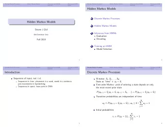
Discrete Markov Process Assume ◮ k states { 1 , . . . , k } ◮ state transition probability a ij = P ( x = j | y = i ) satisfies k � a ij ≥ 0 and a ij = 1 j =1 Given a state sequence { x 1 , . . . , x T } , where x t ∈ { 1 , . . . , k } P ( x 1 , . . . , x T ) = P ( x 1 ) P ( x 2 | x 1 ) . . . P ( x T − 1 | x T ) = π x 1 a x 1 x 2 . . . a x T − 1 x T

Extension to HMM ◮ k state, state transition probability A = { a ij } , initial state distribution Π = { π i } , hidden state sequence X = { x 1 , . . . x T } ◮ observed sequence Y = { y 1 , . . . , y T } , where y T ∈ { 1 , . . . , m } ◮ observation symbol probability B = { b j ( ℓ ) } where b j ( ℓ ) = P ( y t = ℓ | x t = j ) Denote by Λ = ( A , B , Π) the model parameters, then T − 1 T � � P ( X , Y | Λ) = P ( x 1 ) P ( x t +1 | x t ) P ( y t | x t ) t =1 t =1

Three problems of HMM Evaluation: Given observation sequence Y and model parameters Λ, how to compute P ( Y | Λ) Decoding: Given observation Y and model parameters Λ, how to choose the “optimal” hidden state sequence X Learning: How to find the model parameters Λ to maximize P ( Y | Λ)

Problem 1: Evaluation The naive solution. Since it is easy to compute P ( Y , X | Λ), then � P ( Y | Λ) = ( P ( Y , X | Λ)) all possible X However, the time complexity is O ( Tk T ), even for 5 state and 100 observations, there are on the order of 10 72 operations. But HMM is a tree, certainly we can have polynomial algorithms.

The forward procedure Let α t ( i ) = P ( y 1 , . . . , y t , x t = i | Λ) , then k � P ( Y | Λ) = α T ( i ) i =1 α t ( i ) can be computed recursively ∀ i α 1 ( i ) = π i b i ( y 1 ) k � α t +1 ( i ) = P ( y t +1 | x t +1 = i ) P ( x t +1 = i | x t = j ) α t ( j ) j =1   k � = b i ( y t +1 ) a ij α t ( j ) ∀ i , t ≥ 1   j =1

Illustration of the forward procedure α t ( i ) are represented by nodes α 1 ( i ) = π i b i ( y 1 ) ∀ i   k � α t +1 ( i ) = b i ( y t +1 ) a ij α t ( j ) ∀ i , t ≥ 1   j =1

The backward procedure, cont Similar, we can compute in backward way, let β t ( i ) = P ( y t +1 , . . . , y T | x t = i , Λ) then k k � � P ( Y | Λ) = β 1 ( i ) π i = α t ( i ) β t ( i ) ∀ i i =1 i =1 β t ( i ) can be also computed recursively ∀ i β T ( i ) = 1 k � β t ( i ) = P ( y t +1 | x t +1 = j ) P ( x t +1 = j | x t = i ) β t +1 ( j ) j =1 k � = b j ( y t +1 ) a ij β t +1 ( j ) ∀ i , t < T j =1

Problem 2: Decoding There are several possible optimal criteria. One is “individually most likely”. Define the probability of being state i at time t given Y and Λ: γ t ( i ) = P ( x t = i | Y , Λ) , then γ t ( i ) = P ( x t = i , Y | Λ) α t ( i ) β t ( i ) = � k P ( Y | Λ) j =1 α t ( j ) β t ( j ) Choose the individually most likely state x ∗ t = argmax γ t ( i ) i The problem: ignore the sequence structure of X , may select { . . . , i , j , . . . } even if a ij = 0

Viterbi Algorithm The improved criteria is to find the best state sequence argmax P ( X | Y , Λ) = argmax P ( Y , X | Λ) , X X which can be solved by dynamic programming easily. Define δ t ( i ) = x 1 ,..., x t − 1 P ( x 1 , . . . , x t − 1 , x t = i , y 1 , . . . , y t | Λ) max then max P ( Y , X | Λ) = max δ T ( i ) i and δ 1 ( i ) = π i b i ( y 1 ) δ t +1 ( i ) = max P ( y t +1 | x t +1 = i ) P ( x t +1 = i | x t = j ) δ t ( j ) j = max b i ( y t +1 ) a ji δ t ( j ) ∀ t ≥ 1 j

Viterbi Algorithm Given δ t ( i ) = x 1 ,..., x t − 1 P ( x 1 , . . . , x t − 1 , x t = i , y 1 , . . . , y t | Λ) max Further let φ 1 ( i ) = 0 ∀ t ≥ 1 , φ t +1 ( i ) = argmax δ t ( j ) a ji j then the optimal state sequence maximize P ( X | Y , Λ) can be obtained by backtracking x ∗ T = argmax δ T ( i ) i x ∗ t − 1 = φ t ( x ∗ for t = T , T − 1 , . . . t )

Problem 3: Learning ◮ find Λ to maximize P ( Y | Λ) ◮ can be solved by EM algorithm. The objective function is not convex, only a local maximum is guaranteed. Define the prob of being statue i at time t and j at time t + 1 ξ t ( i , j ) = P ( x t = i , x t +1 = j | Y , Λ) = α t ( j ) a ij b j ( y t +1 ) β t +1 ( j ) P ( Y | Λ) α t ( j ) a ij b j ( y t +1 ) β t +1 ( j ) = � i , j α t ( j ) a ij b j ( y t +1 ) β t +1 ( j ) and the prob of being statue i at time t k � γ t ( i ) = ξ t ( i , j ) j =1

Learning, cont Then we have the following update rules. Iterate until converge: π ′ i ← #state i at time 1 = γ 1 ( i ) � T − 1 ij ← #transition from state i to j t =1 ξ t ( i , j ) a ′ = � T − 1 #transition from state i t =1 γ t ( i ) � T yt = ℓ γ t ( i ) t =1 i ( ℓ ) ← #observations of ℓ at state i b ′ = � T #state i t =1 γ t ( i ) ◮ new parameters are still probabilities: k k k � � � π ′ i = 1 , a ′ ij = 1 , b ′ i ( ℓ ) = 1 i =1 j =1 i =1 ◮ non-decreasing: P ( Y | Λ ′ ) ≥ P ( Y | Λ)

HMM variants ◮ Left-right model, namely a ij = 0 for j < i ◮ continuous observations, namely y t is continuous. one convenient assumption Gaussian, P ( y t | x t = i ) = N ( µ i , Σ i ). ◮ auto-regressive HMM

Outline Hidden Markov Model Kalman Filter A Unifying View of Linear Gaussian Models

Basic Idea Kalman Filter, also known as linear dynamic system, is just like an HMM, except the hidden state are continuous. An example: Object Tracking: Estimate motion of targets in 3D world from indirect, potentially noisy measurements

Object Tracking: 2D example ◮ Let x t , 1 , x t , 2 be the object position at time t and x t , 3 , x t , 4 be the corresponding velocity ◮ let ∆ be the sampling period, assume the following random acceleration model:         x t +1 , 1 1 0 ∆ 0 x t , 1 ǫ t , 1 0 1 0 ∆ ǫ t , 2 x t +1 , 2 x t , 2          =  +  ,         x t +1 , 3 0 0 1 0 x t , 3 ǫ t , 3      0 0 0 1 ǫ t , 4 x t +1 , 4 x t , 4 where ǫ t ∼ N (0 , Q ) is the system noise ◮ suppose only positions are observed,   x t , 1 � y t , 1 � � 1 � � δ t , 1 � 0 0 0 x t , 2   =  + ,   y t , 2 0 1 0 0 x t , 3 δ t , 2  x t , 4 where δ t ∼ N (0 , R ) is the measurement noise

Example: Robot Navigation Simultaneous Localization and Mapping (SLAM): as robot moves, estimate its pose and world geometry We will back Kalman Filter later.

Outline Hidden Markov Model Kalman Filter A Unifying View of Linear Gaussian Models

Discrete time linear dynamic with Gaussian noise for each time t = 1 , 2 , . . . , the system generates state x t ∈ R k and observation y t ∈ R p by: w t ∼ N (0 , Q ) x t +1 = Ax t + w t y t = Bx t + v t v t ∼ N (0 , R ) , both w t and v t are temporally white (uncorrelated with t ) if assume the initial state x 1 ∼ N ( π, Q 1 ) then all x t and y t will be Gaussian, x t +1 | x t ∼ N ( Ax t , Q ) y t | x t ∼ N ( Bx t , R )