Topics in Brain Computer Interfaces Topics in Brain Computer - PowerPoint PPT Presentation
Topics in Brain Computer Interfaces Topics in Brain Computer Interfaces CS295- -7 7 CS295 Professor: M ICHAEL B LACK TA: F RANK W OOD Spring 2005 Kalman Filtering Michael J. Black - CS295-7 2005 Brown University v v = + z H x noise
Topics in Brain Computer Interfaces Topics in Brain Computer Interfaces CS295- -7 7 CS295 Professor: M ICHAEL B LACK TA: F RANK W OOD Spring 2005 Kalman Filtering Michael J. Black - CS295-7 2005 Brown University
v v = + z H x noise t t Approximation: Linear Gaussian (generative) model observation model v v Ν ~ ( , ) z H x Q − t j t t … Full covariance Q matrix models correlations between cells. H models how firing rates relate to full kinematic model (position, velocity, and acceleration). … Michael J. Black - CS295-7 2005 Brown University
Bayesian Inference Likelihood Prior ( a priori – (evidence) before the evidence) Posterior ( firing | kinematics ) ( kinematics ) p p = ( kinematics | firing ) p ( firing ) p a posteriori probability normalization constant (after the evidence) (independent of mouth) We infer hand kinematics from uncertain evidence and our prior knowledge of how hands move. Michael J. Black - CS295-7 2005 Brown University
Multi-Modal Likelihood likelihood State (e.g. position) How can we represent this? Michael J. Black - CS295-7 2005 Brown University
Non-Parametric Approximation � We could sample at regular intervals Problems? most samples have low probability – wasted computation How finely to discretize High dimensional space – discretization impractical Michael J. Black - CS295-7 2005 Brown University
Factored Sampling weighted samples = = ( ) ( ) i i {( x , ); 1 ... } Weighted samples S w i N Normalized likelihood: ( ) n = ( z | x ) ( ) p n w t t t N ∑ ( ) i ( z | x ) p t t = 1 i Michael J. Black - CS295-7 2005 Brown University
Monte-Carlo Sampling = = ( ) ( ) i i {( , ); 1 ... } x S w i N Given a weighted sample set Cumulative distribution of weights 1 sample 0 1 N Michael J. Black - CS295-7 2005 Brown University
Bayesian Tracking Bayesian Tracking Posterior over model parameters given an image sequence. = ( x | Z ) p Temporal model (prior) t t ∫ κ ( z x ) ( ( x | x ) ( x | Z )) x p p p d − − − − 1 1 1 1 t t t t t t t Posterior from Likelihood of previous time instant observing the firing rates given the hand kinematics. Monte Carlo integration Michael J. Black - CS295-7 2005 Brown University
Particle Filter Particle Filter ( x | Z ) Posterior p − − 1 1 t t Isard & Blake ‘96 Michael J. Black - CS295-7 2005 Brown University
Particle Filter Particle Filter ( x | Z ) Posterior p − − 1 1 t t sample sample Isard & Blake ‘96 Michael J. Black - CS295-7 2005 Brown University
Particle Filter Particle Filter ( x | Z ) Posterior p − − 1 1 t t sample sample Temporal dynamics ( x | x ) p − 1 t t sample sample Isard & Blake ‘96 Michael J. Black - CS295-7 2005 Brown University
Particle Filter Particle Filter ( x | Z ) Posterior p − − 1 1 t t sample sample Temporal dynamics ( x | x ) p − 1 t t sample sample Likelihood ( z | x ) p t t Isard & Blake ‘96 Michael J. Black - CS295-7 2005 Brown University
Particle Filter Particle Filter ( x | Z ) Posterior p − − 1 1 t t sample sample Temporal dynamics ( x | x ) p − 1 t t sample sample Likelihood ( z | x ) p t t normalize normalize ( x | Z ) p Posterior t t Isard & Blake ‘96 Michael J. Black - CS295-7 2005 Brown University
Pseudocode condense1step % generate cumulative distribution for posterior at t-1 …. % generate a vector of uniform random numbers. % if a the number is greater than refreshRate then % generate a vector of uniform random numbers % use these to search the cumulative probability % find the indices of the corresponding particles % for each of these particles, predict the new state (eg. Add Gaussian noise!) % for each of these new states compute the log likelihood % else generate a particle at random and compute its log likelihood. % find the maximum log likelihood and subtract it from all the other log likelihoods % construct the posterior at time t by exponentiating all the log likelihoods and normalizing so they sum to 1. Michael J. Black - CS295-7 2005 Brown University
Michael Isard Brown University Particle Filter Michael J. Black - CS295-7 2005
Linear Gaussian Likelihood Generative model for the observation: = + z H x q k k k k × ∈ R = c c × q ~ ( 0 , Q ), N ∈ R Q , L c d 1 2 . k , , ,M H , k k k k Michael J. Black - CS295-7 2005 Brown University
Explicit Form The likelihood model is equivalent to that z ~ ( H x , Q ) N k k k k The conditional probability has explicit form: 1 1 − = − − − 1 T ( z x ) exp( ( z H x ) Q ( z H x )) p π k k k k k k k k k 1 / 2 c (( 2 ) det( Q )) 2 k Michael J. Black - CS295-7 2005 Brown University
Linear Gaussian Temporal Prior Temporal prior of the state: = + x A x w − 1 k k k k × = × ∈ R d d ∈ R L w ~ ( 0 , W ), 2 3 , . d d N W , k , M A , k k k k Michael J. Black - CS295-7 2005 Brown University
Explicit Form The prior model is equivalent to that x + ~ ( A x , W ) N 1 k k k k The conditional probability has explicit form: 1 1 − = − − − 1 T ( x x ) exp( ( x A x ) W ( x A x )) p + + + π 1 1 1 k k k k k k k k k 1 / 2 d (( 2 ) det( W )) 2 k Michael J. Black - CS295-7 2005 Brown University
Kalman Filter Model Definition: System Equation: = + x A x w , ∈ w ( 0 , W ) N − 1 k k k k k k = L 2 , 3 , k Measurement Equation: = + ∈ q ( 0 , Q ) N z H x q , k k k k k k = L 1 , 2 , k Assumption: All random variables have Gaussian distributions and they are linearly related Michael J. Black - CS295-7 2005 Brown University
Linear Gaussian Model = ( x | Z ) p t t ∫ κ ( z x ) ( ( x | x ) ( x | Z )) x p p p d − − − − 1 1 1 1 t t t t t t t Some basic facts about Gaussians: Marginal of a Gaussian is Gaussian Gaussian times a Gaussian is Gaussian = µ Σ = µ Σ ( x ) ( , ), ( x ) ( , ) p N p N 1 1 1 2 2 2 = µ Σ ( x ) ( x ) ( , ) p p zN 1 2 3 3 − − µ = Σ Σ µ + Σ µ 1 1 ( ) 3 3 1 1 2 2 − − − Σ = Σ + Σ 1 1 1 ( ) 3 1 2 Michael J. Black - CS295-7 2005 Brown University
Linear Gaussian Model = ( x | Z ) p t t ∫ κ ( z x ) ( ( x | x ) ( x | Z )) x p p p d − − − − 1 1 1 1 t t t t t t t A linear transformation of a Gaussian distributed random variable is also Gaussian: x ~ ( x , Q ) N = + y Ax b + T y ~ ( A x b , AQA ) N Michael J. Black - CS295-7 2005 Brown University
Linear Gaussian Model = ( x | Z ) p t t ∫ κ ( z x ) ( ( x | x ) ( x | Z )) x p p p d − − − − 1 1 1 1 t t t t t t t ( Ax − 1 W , ) ( x , P ) N N − − 1 1 t t t + T x ~ ( A x , AP A W ) N − − 1 1 t t t − − ˆ x ~ ( x , P ) N t t t Michael J. Black - CS295-7 2005 Brown University
Linear Gaussian Model = ( x | Z ) p t t ∫ κ ( z x ) ( ( x | x ) ( x | Z )) x p p p d − − − − 1 1 1 1 t t t t t t t − − ( Hx t , Q ) N ˆ x ~ ( x , P ) N t t t ⎛ ⎞ 1 1 − 1 − − − − × − − − − − − ⎜ ⎟ 1 T T ˆ ˆ exp ( z Hx ) ( z Hx ) ( x x ) P ( x x ) const Q t t t t t t t t t ⎝ ⎠ 2 2 Michael J. Black - CS295-7 2005 Brown University
Linear Gaussian Model ( x | z ) p t t ⎛ ⎞ 1 1 − 1 − − − − = × − − − − − − ⎜ ⎟ 1 T T ˆ ˆ exp ( z Hx ) ( z Hx ) ( x x ) P ( x x ) const Q t t t t t t t t t ⎝ ⎠ 2 2 = ˆ ( x | P ) N t t ( ) ( ) − 1 − − 1 1 = − + − − − + − 1 1 T T ˆ ˆ x P H Q H P x H Q z ( ) t t t t t − 1 − − − = + 1 T ˆ ˆ x P P x H Q z t t t t t ( ) − 1 − 1 − − = + 1 T P P H Q H t t Michael J. Black - CS295-7 2005 Brown University
Linear Gaussian Model ( ) ( ) − 1 − − 1 1 − − − − − = + + 1 1 T T ˆ ˆ x P H Q H P x H Q z t t t t t ( ) − 1 − 1 − − = + 1 T P P H Q H t t Some algebra. − − = + − ˆ ˆ ˆ x x K ( z H x ) t t t t t − = 1 T K P H Q t t ( ) − 1 − 1 − − − = + 1 1 T T K P H Q H H Q t t Michael J. Black - CS295-7 2005 Brown University
Simplifying Matrix inversion lemma ( ) − 1 − 1 − − − = + 1 1 T T K P H Q H H Q t t ( ) − 1 − 1 − − + 1 T P H Q H t − − − − − − = − + 1 1 T T P P H ( Q HP H ) HP t t t t = P t Michael J. Black - CS295-7 2005 Brown University
Recommend
More recommend
Explore More Topics
Stay informed with curated content and fresh updates.


