Markov processes (Markov chains) Construct a Bayes net from these - PDF document

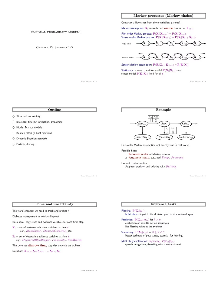
Markov processes (Markov chains) Construct a Bayes net from these variables: parents? Markov assumption: X t depends on bounded subset of X 0: t − 1 Temporal probability models First-order Markov process: P ( X t | X 0: t − 1 ) = P ( X t | X t − 1 ) Second-order Markov process: P ( X t | X 0: t − 1 ) = P ( X t | X t − 2 , X t − 1 ) X t −2 X t −1 X t +1 X t +2 X t First−order Chapter 15, Sections 1–5 X t −2 X t −1 X t X t +1 X t +2 Second−order Sensor Markov assumption: P ( E t | X 0: t , E 0: t − 1 ) = P ( E t | X t ) Stationary process: transition model P ( X t | X t − 1 ) and sensor model P ( E t | X t ) fixed for all t Chapter 15, Sections 1–5 1 Chapter 15, Sections 1–5 4 Outline Example ♦ Time and uncertainty R t −1 P(R ) t t 0.7 f ♦ Inference: filtering, prediction, smoothing 0.3 Rain t −1 Rain t +1 Rain t ♦ Hidden Markov models R P(U ) t t t 0.9 ♦ Kalman filters (a brief mention) f 0.2 Umbrella t −1 Umbrella Umbrella t +1 t ♦ Dynamic Bayesian networks ♦ Particle filtering First-order Markov assumption not exactly true in real world! Possible fixes: 1. Increase order of Markov process 2. Augment state , e.g., add Temp t , Pressure t Example: robot motion. Augment position and velocity with Battery t Chapter 15, Sections 1–5 2 Chapter 15, Sections 1–5 5 Time and uncertainty Inference tasks The world changes; we need to track and predict it Filtering: P ( X t | e 1: t ) belief state—input to the decision process of a rational agent Diabetes management vs vehicle diagnosis Prediction: P ( X t + k | e 1: t ) for k > 0 Basic idea: copy state and evidence variables for each time step evaluation of possible action sequences; like filtering without the evidence X t = set of unobservable state variables at time t e.g., BloodSugar t , StomachContents t , etc. Smoothing: P ( X k | e 1: t ) for 0 ≤ k < t better estimate of past states, essential for learning E t = set of observable evidence variables at time t e.g., MeasuredBloodSugar t , PulseRate t , FoodEaten t Most likely explanation: arg max x 1: t P ( x 1: t | e 1: t ) speech recognition, decoding with a noisy channel This assumes discrete time ; step size depends on problem Notation: X a : b = X a , X a +1 , . . . , X b − 1 , X b Chapter 15, Sections 1–5 3 Chapter 15, Sections 1–5 6

Filtering Smoothing example 0.500 0.627 Aim: devise a recursive state estimation algorithm: 0.500 0.373 True 0.500 0.818 0.883 P ( X t +1 | e 1: t +1 ) = f ( e t +1 , P ( X t | e 1: t )) forward False 0.500 0.182 0.117 0.883 0.883 smoothed 0.117 0.117 P ( X t +1 | e 1: t +1 ) = P ( X t +1 | e 1: t , e t +1 ) 0.690 1.000 backward 0.410 1.000 = α P ( e t +1 | X t +1 , e 1: t ) P ( X t +1 | e 1: t ) = α P ( e t +1 | X t +1 ) P ( X t +1 | e 1: t ) Rain 0 Rain 1 Rain 2 I.e., prediction + estimation. Prediction by summing out X t : P ( X t +1 | e 1: t +1 ) = α P ( e t +1 | X t +1 ) Σ x t P ( X t +1 | x t , e 1: t ) P ( x t | e 1: t ) Umbrella 1 Umbrella 2 = α P ( e t +1 | X t +1 ) Σ x t P ( X t +1 | x t ) P ( x t | e 1: t ) Forward–backward algorithm: cache forward messages along the way f 1: t +1 = Forward ( f 1: t , e t +1 ) where f 1: t = P ( X t | e 1: t ) Time linear in t (polytree inference), space O ( t | f | ) Time and space constant (independent of t ) Chapter 15, Sections 1–5 7 Chapter 15, Sections 1–5 10 Filtering example Most likely explanation Most likely sequence � = sequence of most likely states!!!! 0.500 0.627 0.500 0.373 Most likely path to each x t +1 True 0.500 0.818 0.883 = most likely path to some x t plus one more step False 0.500 0.182 0.117 x 1 ... x t P ( x 1 , . . . , x t , X t +1 | e 1: t +1 ) max Rain 0 Rain 1 Rain 2   = P ( e t +1 | X t +1 ) max  P ( X t +1 | x t ) max x 1 ... x t − 1 P ( x 1 , . . . , x t − 1 , x t | e 1: t )  x t Identical to filtering, except f 1: t replaced by Umbrella 1 Umbrella 2 m 1: t = x 1 ... x t − 1 P ( x 1 , . . . , x t − 1 , X t | e 1: t ) , max I.e., m 1: t ( i ) gives the probability of the most likely path to state i . Update has sum replaced by max, giving the Viterbi algorithm: m 1: t +1 = P ( e t +1 | X t +1 ) max x t ( P ( X t +1 | x t ) m 1: t ) Chapter 15, Sections 1–5 8 Chapter 15, Sections 1–5 11 Smoothing Viterbi example X 1 X 0 X k X t Rain 1 Rain 2 Rain 3 Rain 4 Rain 5 true true true true true E E k E state t 1 space paths false false false false false Divide evidence e 1: t into e 1: k , e k +1: t : true true false true true P ( X k | e 1: t ) = P ( X k | e 1: k , e k +1: t ) umbrella = α P ( X k | e 1: k ) P ( e k +1: t | X k , e 1: k ) .8182 .5155 .0361 .0334 .0210 most = α P ( X k | e 1: k ) P ( e k +1: t | X k ) likely paths .1818 .0491 .1237 .0173 .0024 = α f 1: k b k +1: t m 1:1 m 1:2 m 1:3 m 1:4 m 1:5 Backward message computed by a backwards recursion: P ( e k +1: t | X k ) = Σ x k +1 P ( e k +1: t | X k , x k +1 ) P ( x k +1 | X k ) = Σ x k +1 P ( e k +1: t | x k +1 ) P ( x k +1 | X k ) = Σ x k +1 P ( e k +1 | x k +1 ) P ( e k +2: t | x k +1 ) P ( x k +1 | X k ) Chapter 15, Sections 1–5 9 Chapter 15, Sections 1–5 12

Hidden Markov models Country dance algorithm X t is a single, discrete variable (usually E t is too) Can avoid storing all forward messages in smoothing by running Domain of X t is { 1 , . . . , S } forward algorithm backwards:  0 . 7 0 . 3   f 1: t +1 = α O t +1 T ⊤ f 1: t Transition matrix T ij = P ( X t = j | X t − 1 = i ) , e.g.,     0 . 3 0 . 7  O − 1 t +1 f 1: t +1 = α T ⊤ f 1: t α ′ ( T ⊤ ) − 1 O − 1 t +1 f 1: t +1 = f 1: t Sensor matrix O t for each time step, diagonal elements P ( e t | X t = i )   0 . 9 0  Algorithm: forward pass computes f t , backward pass does f i , b i e.g., with U 1 = true , O 1 =     0 0 . 2  Forward and backward messages as column vectors: f 1: t +1 = α O t +1 T ⊤ f 1: t b k +1: t = TO k +1 b k +2: t Forward-backward algorithm needs time O ( S 2 t ) and space O ( St ) Chapter 15, Sections 1–5 13 Chapter 15, Sections 1–5 16 Country dance algorithm Country dance algorithm Can avoid storing all forward messages in smoothing by running Can avoid storing all forward messages in smoothing by running forward algorithm backwards: forward algorithm backwards: f 1: t +1 = α O t +1 T ⊤ f 1: t f 1: t +1 = α O t +1 T ⊤ f 1: t O − 1 t +1 f 1: t +1 = α T ⊤ f 1: t O − 1 t +1 f 1: t +1 = α T ⊤ f 1: t α ′ ( T ⊤ ) − 1 O − 1 α ′ ( T ⊤ ) − 1 O − 1 t +1 f 1: t +1 = f 1: t t +1 f 1: t +1 = f 1: t Algorithm: forward pass computes f t , backward pass does f i , b i Algorithm: forward pass computes f t , backward pass does f i , b i Chapter 15, Sections 1–5 14 Chapter 15, Sections 1–5 17 Country dance algorithm Country dance algorithm Can avoid storing all forward messages in smoothing by running Can avoid storing all forward messages in smoothing by running forward algorithm backwards: forward algorithm backwards: f 1: t +1 = α O t +1 T ⊤ f 1: t f 1: t +1 = α O t +1 T ⊤ f 1: t O − 1 t +1 f 1: t +1 = α T ⊤ f 1: t O − 1 t +1 f 1: t +1 = α T ⊤ f 1: t α ′ ( T ⊤ ) − 1 O − 1 α ′ ( T ⊤ ) − 1 O − 1 t +1 f 1: t +1 = f 1: t t +1 f 1: t +1 = f 1: t Algorithm: forward pass computes f t , backward pass does f i , b i Algorithm: forward pass computes f t , backward pass does f i , b i Chapter 15, Sections 1–5 15 Chapter 15, Sections 1–5 18

Country dance algorithm Country dance algorithm Can avoid storing all forward messages in smoothing by running Can avoid storing all forward messages in smoothing by running forward algorithm backwards: forward algorithm backwards: f 1: t +1 = α O t +1 T ⊤ f 1: t f 1: t +1 = α O t +1 T ⊤ f 1: t O − 1 t +1 f 1: t +1 = α T ⊤ f 1: t O − 1 t +1 f 1: t +1 = α T ⊤ f 1: t α ′ ( T ⊤ ) − 1 O − 1 α ′ ( T ⊤ ) − 1 O − 1 t +1 f 1: t +1 = f 1: t t +1 f 1: t +1 = f 1: t Algorithm: forward pass computes f t , backward pass does f i , b i Algorithm: forward pass computes f t , backward pass does f i , b i Chapter 15, Sections 1–5 19 Chapter 15, Sections 1–5 22 Country dance algorithm Country dance algorithm Can avoid storing all forward messages in smoothing by running Can avoid storing all forward messages in smoothing by running forward algorithm backwards: forward algorithm backwards: f 1: t +1 = α O t +1 T ⊤ f 1: t f 1: t +1 = α O t +1 T ⊤ f 1: t O − 1 t +1 f 1: t +1 = α T ⊤ f 1: t O − 1 t +1 f 1: t +1 = α T ⊤ f 1: t α ′ ( T ⊤ ) − 1 O − 1 α ′ ( T ⊤ ) − 1 O − 1 t +1 f 1: t +1 = f 1: t t +1 f 1: t +1 = f 1: t Algorithm: forward pass computes f t , backward pass does f i , b i Algorithm: forward pass computes f t , backward pass does f i , b i Chapter 15, Sections 1–5 20 Chapter 15, Sections 1–5 23 Country dance algorithm Kalman filters Can avoid storing all forward messages in smoothing by running Modelling systems described by a set of continuous variables, e.g., tracking a bird flying— X t = X, Y, Z, ˙ X, ˙ Y , ˙ Z . forward algorithm backwards: Airplanes, robots, ecosystems, economies, chemical plants, planets, . . . f 1: t +1 = α O t +1 T ⊤ f 1: t O − 1 t +1 f 1: t +1 = α T ⊤ f 1: t X X t t +1 α ′ ( T ⊤ ) − 1 O − 1 t +1 f 1: t +1 = f 1: t X X Algorithm: forward pass computes f t , backward pass does f i , b i t t +1 Z Z t t +1 Gaussian prior, linear Gaussian transition model and sensor model Chapter 15, Sections 1–5 21 Chapter 15, Sections 1–5 24