Max-Margin Markov Networks Ben Taskar Carlos Guestrin Daphne - PDF document
Max-Margin Markov Networks Ben Taskar Carlos Guestrin Daphne Koller Main Contribution The authors combine a graphic model and a discriminative model and apply it in a sequential learning setting. Graphic models: better at
Max-Margin Markov Networks Ben Taskar Carlos Guestrin Daphne Koller Main Contribution • The authors combine a graphic model and a discriminative model and apply it in a sequential learning setting. – Graphic models: better at interpreting data, worse performance – Discriminative models: better performance, unintelligible working mechanism 1
SVM • SVM officially proposed as a QP problem • Schematic plot SVM (2) • Having learned w, our discriminant function is defined as h( x ) = sign( w · x + b) • One way to extend binary to multiclass SVM is to train a weight vector w for each class, and h( x ) = argmax r (w r *x + b r ), r = 1..k 2
SVM (3) • Multiclass SVM (Crammer & Singer) where M is the matrix with w r (M r ) as row vectors • Scaling problem This QP problem might be much harder to solve. Platt proposed Sequential Minimal Optimization (SMO) to speed up the training. Problem Setting • Multi-class Sequential Supervised Learning – Training example: (X,Y) where • X = (x 1 , …, x T ) is a sequence of feature vectors • Y = (y 1 , …, y T ) is a matching sequence of class labels – Goal: Given new X, predict new Y • We work on OCR data, e.g. 3
Problem Setting (2) • The task is to learn a function from a training set , where with . Given n basis function , h w is defined as: • Note that # of assignments to y is exponential ( k l ). Both representing f j and solving the above argmax are infeasible Graphic Model • Pairwise Markov network – Defined as a graph G = (Y, E); each edge (i,j) associated with a potential Ψ ij (x,yi,yj). – Encodes a joint cpd – Captures interactions between Y’s compactly – Given cpd, intuitively we want to take argmax y P ( y | x ) as our prediction. 4
Unifying Markov Network and SVM • Markov network distribution is a log-linear model • Potential Ψ ij (x,y i ,y j ) can be represented (in log-space) a sum of basis functions over x, y i and y j . • If we define We end up with argmax y P ( y | x ) = argmax y w T f ( x, y ) Formulating SVM • Single-label Multi-class SVM where • This is essentially the same as constraining the margin to be a constant and minimize || w || 5
Formulating SVM (2) • γ -multi-label margin: where • Multi-label SVM • The result of using # of individual labeling errors as loss function. • The QP form: Formulating SVM (3) • Final form (w/ slack variables) • Its dual formulation 6
SMO learning of M 3 Networks • SMO is an efficient algorithm solving QP problems, it has three components – An analytic method to solve two Lagrangian multipliers subproblems – A heuristic for choosing which multipliers to optimize – A method for computing b • We explore the structure of the dual form and propose how to do SMO learning on M 3 networks Generalization Error Bound • A theoretical analysis to relate training error to testing (generalization) error. • Average per label loss • γ -margin per-label loss • Theorem 6.1 …there exists a constant K , the following holds with probability 1- 7
Experiments • We select a subset of ~6100 handwritten words, with average length of ~8 characters, from 150 human subjects • Each word is divided into characters, rasterized into 16x8 images • 26-class problem: {a..z} Experiments (2) • Result – LR – independent-labeling; trained on conditional likelihood – CRF – sequential-labeling; links between yi and yi+1 – SVMs – linear, quadratic and cubic kernels – Multi-class SVM – independent-labeling 8
Recommend
More recommend
Explore More Topics
Stay informed with curated content and fresh updates.
