
On Convergence-Diagnostic based Step Sizes for Stochastic Gradient - PowerPoint PPT Presentation
On Convergence-Diagnostic based Step Sizes for Stochastic Gradient Descent Aymeric Dieuleveut CMAP, cole Polytechnique, Institut Polytechnique de Paris Joint work with Scott Pesme and Nicolas Flammarion (EPFL) 10/03/2020 Cirm Luminy -
On Convergence-Diagnostic based Step Sizes for Stochastic Gradient Descent Aymeric Dieuleveut CMAP, École Polytechnique, Institut Polytechnique de Paris Joint work with Scott Pesme and Nicolas Flammarion (EPFL) 10/03/2020 Cirm Luminy - Optimization for Machine Learning
On Convergence-Diagnostic based Step Sizes for Stochastic Gradient Descent Aymeric Dieuleveut CMAP, École Polytechnique, Institut Polytechnique de Paris Joint work with Scott Pesme and Nicolas Flammarion (EPFL) 10/03/2020 Cirm Luminy - Optimization for Machine Learning 1 / 47
Questions 1. Feel free to ask any question. 2. Let me ask a few ones first: • Who knows about Stochastic Gradient Descent? • Who knows the convergence rate for the last iterate instead of the averaged iterate? • Who knows about Pflug’s convergence diagnosis? 2 / 47
Why would we still talk about SGD ? Objective function f : D → R to minimize � � θ n + 1 = θ n − γ n + 1 f ′ f ′ ( θ n ) + ξ n + 1 ( θ n ) n + 1 ( θ n ) = θ n − γ n + 1 . What choice for the learning rate ( γ n ) n ∈ N ? As often: • Theoreticians ( ♥ ) came up with optimal answers (convex setting). • Practitioners do not use them ! If it works in theory it also works in practice – in theory. Why not? 1. Step size in SGD often depends on unknown parameters (esp. µ -strong convexity). 2. May be very sensitive to those parameters. 3. Does not adapt to the noise and function regularity. 3 / 47
A few observations a) Large learning rates often converge faster at the beginning b) But then results in saturation: two phases behavior. c) Theory suggests to use the Polyak-Ruppert averaged iterate, but the final one might not be that bad. d) In Deep Learning, common practice is to use a constant learning rate, reduced occasionally. 4 / 47
a) Large learning rates often converge faster at the beginning SGD nearly always results in a Bias (initial condition) - Variance (noise) tradeoff. A large initial learning rate maximizes the decay of the bias. -0.5 -1 -1.5 -1 -2 -1.5 -2.5 -3 -2 -3.5 -2.5 1/R 2 1 / 2 R 2 -4 1 / 2 R 2 √ n Decaying Steps -4.5 -3 0 2 4 6 1 2 3 4 5 6 Figure 1: Logistic regression on the Covertype Dataset / Synthetic Dataset 5 / 47
b) Saturation and limit distribution: two phases • “Transient phase" during which the initial conditions are forgotten exponentially fast. • "Stationary phase" where the iterates oscillate around θ ∗ Synthetic logistic dataset d = 2 Synthetic logistic dataset d = 2 0.5 10 −1 1 / 128 R 2 transient θ n θ n transient 1 / 128 R 2 stationnary 0.4 θ n stationnary averaged 10 −2 θ 0 θ * 0.3 10 −3 f ( θ n ) − f ( θ * ) 0.2 10 −4 0.1 10 −5 0.0 10 −6 −0.1 0.0 0.2 0.4 0.6 0.8 1.0 10 0 10 1 10 2 10 3 10 4 10 5 10 6 iteration n Figure 2: Constant step size SGD (2 dimensionnal) path illustration. ( d ) For smooth and strongly convex functions, θ n � π γ , “limit distribution”. π γ is a stationary distribution. 6 / 47
c) Polyak-Ruppert averaged iterate vs final one. Instead of just the final iterate θ ( γ ) n , we can consider the PR-averaged: n − 1 n = 1 � θ ( γ ) θ ( γ ) ¯ k . n k = 0 � Strongly reduces the impact of the noise. � Slows down the Bias term. How bad is the last iterate...? It depends! 7 / 47
c) Polyak-Ruppert averaged iterate vs final one. 2 Final Iterate Average Convex & Smooth Strongly convex & Smooth No noise (deterministic) Finite dimensional quadratic Kernel Regression The Proof by Shamir & Zhang is nice ! 8 / 47
c) Polyak-Ruppert averaged iterate vs final one. 2 9 / 47
Previous work: with decreasing step-sizes (Moulines & Bach 2011), smooth + strongly convex 1 Setting γ n = µ n we get � 1 � �� � 2 � � θ n − θ ∗ � E = O . µ 2 n (Shamir & Zhang 2012), bounded gradients + strongly convex 1 Setting γ n = µ n we get � log( n ) � � � f ( θ n ) − f ( θ ∗ ) = O . E µ n (Shamir & Zhang 2012), bounded gradients + weakly convex 1 Setting γ n = � n we get � log( n ) � � � f ( θ n ) − f ( θ ∗ ) = O . E � n 10 / 47
d) Deep Learning: training NN (1 - test_accuracy) ━ classical_1_wdb learning rate divided by 10 Figure 3: Typical accuracy curve in deep learning (Cifar10 dataset, Resnet18). 11 / 47
Overall... • in the strongly convex case, µ is often unknown and hard to evaluate. • a slight misspecification of µ can lead to arbitrarily slow convergence rates (see Moulines & Bach 2011) • we would like to make use of the uniform convexity assumption • ideally we would like a learning rate sequence that adapts to f • these stepsize sequences are not used in practice for deep learning 12 / 47
Outline Natural strategy: decrease learning rate when no more progress Hopes: adaptive “restarts” to • use “maximal step size” as long as useful • adapt to unknown parameters. Outline: 1. Convergence properties of SGD with piecewise constant learning rates. 2. Detecting Stationarity: Pflug’s Statistic 3. Detecting Stationarity: new heuristic. “Restart” : nothing to restart, just changing the learning rate ! 13 / 47
“Omniscient strategies”. What can we achieve with piecewise constant step sizes ?
What rate can you get if you use a large step size for as long as possible and you decrease it when the loss saturates ? 14 / 47
Oracle algorithm Theorem (Needell 2014) �� � 2 � � θ n − θ ∗ � ≤ (1 − b γ ) n � � θ 0 − θ ∗ � � 2 + c σ 2 γ + O ( γ 2 ), E � � ξ ( θ ∗ ) � 2 � . where b , c depend on f and σ 2 = E Theoretical procedure: Let p , r ∈ [0,1] . Start with l.r. γ 0 , stop at ∆ n 1 : σ 2 �� � 2 � �� � 2 � � θ n − θ ∗ � � θ 0 − θ ∗ � [1 − 2 γ 0 µ ] n E µ γ 0 . E ≤ + � �� � � �� � ∆ n 1 s . t ( ) = p × ( ) Set γ 1 = r γ 0 and restart from θ n 1 = θ ∆ n 1 : σ 2 �� � 2 � �� � 2 � � θ n − θ ∗ � � θ n 1 − θ ∗ � ≤ [1 − 2 γ 1 µ ] ( n − n 1 ) E E + µ γ 1 . � �� � � �� � ∆ n 2 s . t ( ) = p × ( ) etc. (Related but slightly different from Hazan Kale 2010, e.g.) 15 / 47
Oracle algorithm analysis, good news Theorem ( Strongly convex + smooth ) Following the previous oracle procedure and assuming that � θ 0 − θ ∗ � 2 ≤ ( p + 1) σ 2 µ γ 0 : ≤ ( p + 1) σ 2 � � �� � 2 � (1 + 1 p ) 1 1 � θ n k − θ ∗ � 1 − r ln . E µ 2 n k µ r � � 1 ≤ O µ 2 n k • The upper bound can be optimized over p and r • Purely theoretical result since none of these constants are known. • The step size sequence produced is piecewise constant and ’imitates’ γ n = 1/ µ n . Beyond the Smooth & Strongly convex : uniformly convex functions 16 / 47
Assumptions on f Convexity: • Weak convexity: f ( θ 1 ) ≥ f ( θ 2 ) +〈 f ′ ( θ 2 ), θ 1 − θ 2 〉 • Strong convexity, µ > 0 : f ( θ 1 ) ≥ f ( θ 2 ) +〈 f ′ ( θ 2 ), θ 1 − θ 2 〉+ µ 2 � θ 1 − θ 2 � 2 • Uniform convexity : f is uniformly convex with parameters µ > 0 , ρ ∈ [2, +∞ [ if: f ( θ 1 ) ≥ f ( θ 2 ) +〈 f ′ ( θ 2 ), θ 1 − θ 2 〉+ µ ρ � θ 1 − θ 2 � ρ . Smoothness: • (L-smoothness) for any n ∈ N , f n is L-smooth: � � � f ′ n ( θ 1 ) − f ′ � ≤ L � θ 1 − θ 2 � a.s. n ( θ 2 ) • (Non-smooth, bounded gradients) bounded gradients framework: �� � 2 � � � f ′ ≤ G 2 n ( θ n − 1 ) E 17 / 47
Non-smooth, uniformly convex setting Proposition (PDF 2020) If f is a uniformly convex function with parameter ρ > 2 with G -bounded gradients then: � 1 � 1/ τ � � + G 2 log( n ) γ f ( θ n ) − f ( θ ∗ ) ≤ C E γ n Where τ = 1 − 2 ρ ∈ [0,1] In the finite horizon framework, this results in: � log N � � � f ( θ n ) − f ( θ ∗ ) E ≤ O N 1/(1 + τ ) 1 Notice that 1 + τ ∈ [0.5,1] , we have an interpolation between the weakly convex and strongly convex cases. • Juditsky Nesterov 2014 have a similar rate with a different algorithm • Roulet et d’Aspremont have the N − 1/ τ rate for GD. 18 / 47
Restart at saturation Considering the previous upper bound: and following the previous “oracle” procedure (restart when Bias = p × Var ) Theorem (PDF 20) � � 1 − f ( θ n k ) − f ( θ ∗ ) ≤ O 1 + τ log( n k ) n k As before, the strategy of constant steps with “restart at saturation” gives satisfying rates (as good as the best known strategy for decaying steps) 19 / 47
Numerical simulation in the quadratic case Synthetic LS SGD, oracle piecewise constant, r = 1/4 10 0 10 −1 10 −2 f ( θ n ) − f ( θ * ) 10 −3 10 −4 milestones 1 / 2 R 2 10 −5 piecewise constant 10 0 10 1 10 2 10 3 10 4 10 5 10 6 iteration n Figure 4: Oracle constant piece wise SGD 20 / 47
Recommend


More recommend
Explore More Topics
Stay informed with curated content and fresh updates.