Markov Chains Toolbox Search: uninformed/heuristic Adversarial - PowerPoint PPT Presentation
Markov Chains Toolbox Search: uninformed/heuristic Adversarial search Probability Bayes nets Naive Bayes classifiers Reasoning over time In a Bayes net, each random variable (node) takes on one specific value. Good for
Markov Chains
Toolbox • Search: uninformed/heuristic • Adversarial search • Probability • Bayes nets – Naive Bayes classifiers
Reasoning over time • In a Bayes net, each random variable (node) takes on one specific value. – Good for modeling static situations. • What if we need to model a situation that is changing over time?
Example: Comcast • In 2004 and 2007, Comcast had the worst customer satisfaction rating of any company or gov't agency, including the IRS. • I have cable internet service from Comcast, and sometimes my router goes down. If the router is online, it will be online the next day with prob=0.8. If it's offline, it will be offline the next day with prob=0.4. • How do we model the probability that my router will be online/offline tomorrow? In 2 days?
Example: Waiting in line • You go to the Apple Store to buy the latest iPhone. Every minute, the first person in line is served with prob=0.5. • Every minute, a new person joins the line with probability 1 if the line length=0 2/3 if the line length=1 1/3 if the line length=2 0 if the line length=3 • How do we model what the line will look like in 1 minute? In 5 minutes?
Markov Chains • A Markov chain is a type of Bayes net with a potentially infinite number of variables (nodes). • Each variable describes the state of the system at a given point in time (t). X 0 X 1 X 2 X 3
Markov Chains • Markov property: P(X t | X t-1 , X t-2 , X t-3 , …) = P(X t | X t-1 ) • Probabilities for each variable are identical: P(X t | X t-1 ) = P(X 1 | X 0 ) X 0 X 1 X 2 X 3
Markov Chains • Since these are just Bayes nets, we can use standard Bayes net ideas. – Shortcut notation: X i:j will refer to all variables X i through X j , inclusive. • Common questions: – What is the probability of a specific event happening in the future? – What is the probability of a specific sequence of events happening in the future?
An alternate formulation • We have a set of states, S. • The Markov chain is always in exactly one state at any given time t. • The chain transitions to a new state at each time t+1 based only on the current state at time t. p ij = P(X t+1 = j | X t = i) • Chain must specify p ij for all i and j, and starting probabilities for P(X 0 = j) for all j.
Two different representations • As a Bayes net: X 0 X 1 X 2 X 3 • As a state transition diagram (similar to a DFA/NFA): S2 S1 S3
Formulate Comcast in both ways • I have cable internet service from Comcast, and sometimes my router goes down. If the router is online, it will be online the next day with prob=0.8. If it's offline, it will be offline the next day with prob=0.4. • Let’s draw this situation in both ways. • Assume on day 0, probability of router being down is 0.5.
Comcast • What is the probability my router is offline for 3 days in a row (days 0, 1, and 2)? – P(X 0 =off, X 1 =off, X 2 =off)? – P(X 0 =off) * P(X 1 =off|X 0 =off) * P(X 2 =off|X 1 =off) – P(X 0 =off) * p off,off * p off,off t Y P ( x 0: t ) = P ( x 0 ) P ( x i | x i − 1 ) i =1
More Comcast • Suppose I don’t know if my router is online right now (day 0). What is the prob it is offline tomorrow? – P(X 1 =off) – P(X 1 =off) = P(X 1 =off, X 0 =on) + P(X 1 =off, X 0 =off) – P(X 1 =off) = P(X 1 =off|X 0 =on) * P(X 0 =on) + P(X 1 =off|X 0 =off) * P(X 0 =off) X P ( X t +1 ) = P ( X t +1 | x t ) P ( x t ) x t
More Comcast • Suppose I don’t know if my router is online right now (day 0). What is the prob it is offline the day after tomorrow ? – P(X 2 =off) – P(X 2 =off) = P(X 2 =off, X 1 =on) + P(X 2 =off, X 1 =off) – P(X 2 =off) = P(X 2 =off|X 1 =on) * P(X 1 =on) + P(X 2 =off|X 1 =off) * P(X 1 =off) X P ( X t +1 ) = P ( X t +1 | x t ) P ( x t ) x t
Markov chains with matrices • Define a transition matrix for the chain: 0 . 8 � 0 . 2 T = 0 . 6 0 . 4 • Each row of the matrix represents the transition probabilities leaving a state. • Let v t = a row vector representing the probability that the chain is in each state at time t. • v t = v t-1 * T
Mini-forward algorithm • Suppose we are given the values of X 0 , X 1 , ... X t , and we want to know X t+1 . • P(X t+1 | X 0 , X 1 , ..., X t ) • Row vector v 0 = P(X 0 ) • v 1 = v 0 * T • v 2 = v 1 * T = v 0 * T * T = v 0 * T 2 • v 3 = v 0 * T 3 • v t = v 0 * T t
Back to the Apple Store... • You go to the Apple Store to buy the latest iPhone. Every minute, the first person in line is served with prob=0.5. • Every minute, a new person joins the line with probability 1 if the line length=0 2/3 if the line length=1 1/3 if the line length=2 0 if the line length=3 • Model this as a Markov chain, assuming the line starts empty. Draw the state transition diagram. • What is T? What is v 0 ?
• Markov chains are pretty easy! • But sometimes they aren't realistic… • What if we can't directly know the states of the model, but we can see some indirect evidence resulting from the states?
Weather • Regular Markov chain – Each day the weather is rainy or sunny. – P(X t = rain | X t-1 = rain) = 0.7 – P(X t = sunny| X t-1 = sunny) = 0.9 • Twist: – Suppose you work in an office with no windows. All you can observe is weather your colleague brings their umbrella to work.
Hidden Markov Models X 0 X 1 X 2 X 3 E 1 E 2 E 3 • The X's are the state variables (never directly observed). • The E's are evidence variables.
Common real-world uses • Speech processing: – Observations are sounds, states are words. • Localization: – Observations are inputs from video cameras or microphones, state is the actual location. • Video processing (example): – Extracting a human walking from each video frame. Observations are the frames, states are the positions of the legs.
Hidden Markov Models X 0 X 1 X 2 X 3 E 1 E 2 E 3 • P(X t | X t-1 , X t-2 , X t-3 , …) = P(X t | X t-1 ) • P(X t | X t-1 ) = P(X 1 | X 0 ) • P(E t | X 0:t , E 0:t-1 ) = P(E t | X t ) • P(E t | X t ) = P(E 1 | X 1 )
Hidden Markov Models X 0 X 1 X 2 X 3 E 1 E 2 E 3 • What is P(X 0:t , E 1:t )? t Y P ( X 0 ) P ( X i | X i − 1 ) P ( E i | X i ) i =1
Common questions • Filtering : Given a sequence of observations, what is the most probable current state? – Compute P(X t | e 1:t ) • Prediction : Given a sequence of observations, what is the most probable future state? – Compute P(X t+k | e 1:t ) for some k > 0 • Smoothing : Given a sequence of observations, what is the most probable past state? – Compute P(X k | e 1:t ) for some k < t
Common questions • Most likely explanation: Given a sequence of observations, what is the most probable sequence of states? – Compute argmax P ( x 1: t | e 1: t ) x 1: t • Learning : How can we estimate the transition and sensor models from real-world data? (Future machine learning class?)
Hidden Markov Models R 0 R 1 R 2 R 3 U 1 U 2 U 3 • P(R t = yes | R t-1 = yes) = 0.7 P(R t = yes | R t-1 = no) = 0.1 • P(U t = yes | R t = yes) = 0.9 P(U t = yes | R t = no) = 0.2
Filtering • Filtering is concerned with finding the most probable "current" state from a sequence of evidence. • Let's compute this.
Forward algorithm • Recursive computation of the probability distribution over current states. • Say we have P(X t | e 1:t ) P ( X t +1 | e 1: t +1 ) = X α P ( e t +1 | X t +1 ) P ( X t +1 | x t ) P ( x t | e 1: t ) x t
Forward algorithm • Markov chain version: X P ( X t +1 ) = P ( X t +1 | x t ) P ( x t ) x t • Hidden Markov model version: P ( X t +1 | e 1: t +1 ) = X α P ( e t +1 | X t +1 ) P ( X t +1 | x t ) P ( x t | e 1: t ) x t
Forward algorithm • Today is Day 2, and I've been pulling all- nighters for two days! • My colleague brought their umbrella on days 1 and 2. • What is the probability it is raining today?
Matrices to the rescue! • Define a transition matrix T as normal. • Define a sequence of observation matrices O 1 through O t . • Each O matrix is a diagonal matrix with the entries corresponding to that particular observation given each state. f 1: t +1 = α f 1: t · T · O t +1 where each f is a row vector containing the probability distribution at state t.
f1:0=[0.5, 0.5] f1:1=[0.75, 0.25] f1:2=[0.846, 0.154] T = [0.7, 0.3] R1 R0 R2 [0.1, 0.9] O1 = [0.9, 0.0] [0.0, 0.2] U1 U2 O2 = [0.9, 0.0] [0.0, 0.2] f1:0 = P(R0) = [0.5, 0.5] f1:1 = P(R1 | u1) = 𝛃 * f1:0 * T * O1 = 𝛃 [0.36, 0.12] = [0.75, 0.25] f1:2 = P(R2 | u1, u2) = 𝛃 * f1:1 * T * O2 = 𝛃 [0.495, 0.09] = [.846, .154]
Forward algorithm • Note that the forward algorithm only gives you the probability of X t taking into account evidence at times 1 through t. • In other words, say you calculate P(X 1 | e 1 ) using the forward algorithm, then you calculate P(X 2 | e 1 , e 2 ). – Knowing e2 changes your calculation of X1. – That is, P(X 1 | e 1 ) != P(X 1 | e 1 , e 2 )
Backward algorithm • Updates previous probabilities to take into account new evidence. • Calculates P(X k | e 1:t ) for k < t – aka smoothing.
Backward matrices • Main equations: b k : t = T · O k · b k +1: t (column vec of 1s) b t +1: t = [1; · · · ; 1] P ( X k | e 1: t ) = α f 1: k × b k +1: t
Recommend
More recommend
Explore More Topics
Stay informed with curated content and fresh updates.
