CSE 473: Artificial Intelligence Spring 2014 Markov Models Hanna - PowerPoint PPT Presentation
CSE 473: Artificial Intelligence Spring 2014 Markov Models Hanna Hajishirzi Many slides adapted from Pieter Abbeel, Dan Klein, Dan Weld,Stuart Russell, Andrew Moore & Luke Zettlemoyer 1 Markov Chains !
CSE 473: Artificial Intelligence Spring 2014 Markov Models Hanna Hajishirzi Many slides adapted from Pieter Abbeel, Dan Klein, Dan Weld,Stuart Russell, Andrew Moore & Luke Zettlemoyer 1
Markov Chains ! OZen,#we#want#to#reason#about#a#sequence#of#observa8ons# ! Speech#recogni8on# ! Robot#localiza8on# ! User#a:en8on# ! Medical#monitoring# ! Need#to#introduce#8me#(or#space)#into#our#models# 2
Markov Models (Markov Chains) § A Markov model is: § a MDP with no actions (and no rewards) X 1 X 2 X 3 X 4 X N § A Markov model includes: § Random variables X t for all time steps t (the state) § Parameters: called transition probabilities or dynamics, specify how the state evolves over time (also, initial probs) and
Markov Models (Markov Chains) X 1 X 2 X 3 X 4 X N § A Markov model defines § a joint probability distribution: P ( X 1 , X 2 , X 3 , X 4 ) = P ( X 1 ) P ( X 2 | X 1 ) P ( X 3 | X 2 ) P ( X 4 | X 3 ) ! More#generally:# P ( X 1 , X 2 , . . . , X T ) = P ( X 1 ) P ( X 2 | X 1 ) P ( X 3 | X 2 ) . . . P ( X T | X T − 1 ) § One common inference problem: § Compute marginals P(X t ) for all time steps t
Markov Model X 1 X 2 X 3 X 4 X N ! Ques8ons#to#be#resolved:# ! Does#this#indeed#define#a#joint#distribu8on?# ! Can#every#joint#distribu8on#be#factored#this#way,#or#are#we#making#some#assump8ons# about#the#joint#distribu8on#by#using#this#factoriza8on?# 5
Chain Rule and Markov Models P ( X 1 , X 2 , X 3 , X 4 ) = P ( X 1 ) P ( X 2 | X 1 ) P ( X 3 | X 2 ) P ( X 4 | X 3 ) X 1 X 2 X 3 X 4 ! From#the#chain#rule,#every#joint#distribu8on#over#################################can#be#wri:en#as:# X 1 , X 2 , X 3 , X 4 P ( X 1 , X 2 , X 3 , X 4 ) = P ( X 1 ) P ( X 2 | X 1 ) P ( X 3 | X 1 , X 2 ) P ( X 4 | X 1 , X 2 , X 3 ) ! Assuming#that# ####################################################################and# ⊥ X 1 | X 2 ⊥ X 1 , X 2 | X 3 X 3 ⊥ X 4 ⊥ ####results#in#the#expression#posited#on#the#previous#slide:## P ( X 1 , X 2 , X 3 , X 4 ) = P ( X 1 ) P ( X 2 | X 1 ) P ( X 3 | X 2 ) P ( X 4 | X 3 ) 6
Chain Rule and Markov Models X 1 X 2 X 3 X 4 ! From#the#chain#rule,#every#joint#distribu8on#over#########################################can#be#wri:en#as:# X 1 , X 2 , . . . , X T T Y P ( X 1 , X 2 , . . . , X T ) = P ( X 1 ) P ( X t | X 1 , X 2 , . . . , X t − 1 ) t =2 ! Assuming#that#for#all# t :## ⊥ X 1 , . . . , X t − 2 | X t − 1 X t ⊥ ####gives#us#the#expression#posited#on#the#earlier#slide:## T Y P ( X 1 , X 2 , . . . , X T ) = P ( X 1 ) P ( X t | X t − 1 ) t =2 7
Conditional Independence X 1 X 2 X 3 X 4 § Basic conditional independence: § Past and future independent of the present § Each time step only depends on the previous § This is called the (first order) Markov property
Implied Conditional Independencies X 1 X 2 X 3 X 4 ! We#assumed:#################################and# ⊥ X 1 | X 2 ⊥ X 1 , X 2 | X 3 X 3 ⊥ X 4 ⊥ ! Do#we#also#have # # # # #?# ⊥ X 3 , X 4 | X 2 X 1 ⊥ ! Yes!## P ( X 1 | X 2 , X 3 , X 4 ) = P ( X 1 , X 2 , X 3 , X 4 ) ! Proof:# P ( X 2 , X 3 , X 4 ) P ( X 1 ) P ( X 2 | X 1 ) P ( X 3 | X 2 ) P ( X 4 | X 3 ) = P x 1 P ( x 1 ) P ( X 2 | x 1 ) P ( X 3 | X 2 ) P ( X 4 | X 3 ) = P ( X 1 , X 2 ) P ( X 2 ) = P ( X 1 | X 2 ) 9
Markov Models (Recap) ! Explicit#assump8on#for#all### t #:# ⊥ X 1 , . . . , X t − 2 | X t − 1 X t ⊥ ! Consequence,#joint#distribu8on#can#be#wri:en#as:## P ( X 1 , X 2 , . . . , X T ) = P ( X 1 ) P ( X 2 | X 1 ) P ( X 3 | X 2 ) . . . P ( X T | X T − 1 ) T Y = P ( X 1 ) P ( X t | X t − 1 ) t =2 ! Implied#condi8onal#independencies:##(try#to#prove#this!)# ! Past#variables#independent#of#future#variables#given#the#present# i.e.,#if#####################or######################then:# ⊥ X t 3 | X t 2 X t 1 ⊥ t 1 < t 2 < t 3 t 1 > t 2 > t 3 ! Addi8onal#explicit#assump8on:#########################is#the#same#for#all# t0 P ( X t | X t − 1 ) 10
Example: Markov Chain § Weather: 0.9 0.1 § States: X = {rain, sun} § Transitions: rain sun 0.1 This is a 0.9 conditional distribution § Initial distribution: 1.0 sun § What’s the probability distribution after one step?
Markov Chain Inference § Question: probability of being in state x at time t? § Slow answer: § Enumerate all sequences of length t which end in s § Add up their probabilities …
Mini-Forward Algorithm § Question: What’s P(X) on some day t? § We don’t need to enumerate every sequence! sun sun sun sun rain rain rain rain Forward simulation
0.9 0.1 Example 0.9 rain sun 0.1 § From initial observation of sun P(X 1 ) P(X 2 ) P(X 3 ) P(X ∞ ) § From initial observation of rain P(X 1 ) P(X 2 ) P(X 3 ) P(X ∞ )
Stationary Distributions § If we simulate the chain long enough: § What happens? § Uncertainty accumulates § Eventually, we have no idea what the state is! § Stationary distributions: § For most chains, the distribution we end up in is independent of the initial distribution § Called the stationary distribution of the chain § Usually, can only predict a short time out
Stationary Distributions 0.9 0.1 0.9 rain sun ! Ques8on:#What’s#P(X)#at#8me#t#=#infinity?# 0.1 X 1 X 2 X 3 X 4 P ∞ ( sun ) = P ( sun | sun ) P ∞ ( sun ) + P ( sun | rain ) P ∞ ( rain ) P ∞ ( rain ) = P ( rain | sun ) P ∞ ( sun ) + P ( rain | rain ) P ∞ ( rain ) P ∞ ( sun ) = 0 . 9 P ∞ ( sun ) + 0 . 3 P ∞ ( rain ) 0.1 P ∞ ( rain ) = 0 . 1 P ∞ ( sun ) + 0 . 7 P ∞ ( rain ) 0.9 P ∞ ( sun ) = 3 P ∞ ( rain ) P ∞ ( rain ) = 1 / 3 P ∞ ( sun ) 0.5 P ∞ ( sun ) = 3 / 4 Also:# 0.5 P ∞ ( rain ) = 1 / 4 P ∞ ( sun ) + P ∞ ( rain ) = 1 16
Pac-man Markov Chain Pac-man knows the ghost’s initial position, but gets no observations!
Web Link Analysis § PageRank over a web graph § Each web page is a state § Initial distribution: uniform over pages § Transitions: § With prob. c, follow a random outlink (solid lines) § With prob. 1-c, uniform jump to a random page (dotted lines, not all shown)
PageRank § Stationary distribution § Will spend more time on highly reachable pages § E.g. many ways to get to the Acrobat Reader download page § Somewhat robust to link spam § Google 1.0 returned the set of pages containing all your keywords in decreasing rank, now all search engines use link analysis along with many other factors (rank actually getting less important over time) 19
Recommend
More recommend
Explore More Topics
Stay informed with curated content and fresh updates.
