Markov Chains and Hidden Markov Models COMP 571 - Spring 2015 Luay - PowerPoint PPT Presentation
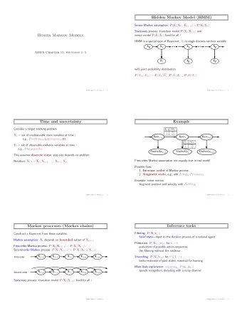
Markov Chains and Hidden Markov Models COMP 571 - Spring 2015 Luay Nakhleh, Rice University Markov Chains and Hidden Markov Models Modeling the statistical properties of biological sequences and distinguishing regions based on these models
Markov Chains and Hidden Markov Models COMP 571 - Spring 2015 Luay Nakhleh, Rice University
Markov Chains and Hidden Markov Models Modeling the statistical properties of biological sequences and distinguishing regions based on these models For the alignment problem, they provide a probabilistic framework for aligning sequences
Example: CpG Islands Regions that are rich in CG dinucleotide Promoter and “ start” regions of many genes are characterized by high frequency of CG dinucleotides (in fact, more C and G nucleotides in general)
CpG Islands: Two Questions Q1: Given a short sequence, does it come from a CpG island? Q2: Given a long sequence, how would we find the CpG islands in it?
CpG Islands Answer to Q1: Given sequence x and probabilistic model M of CpG islands, compute p= P (x|M) If p is “ significant” , then x comes from a CpG island; otherwise, x does not come from a CpG island
CpG Islands Answer to Q1: Given sequence x, probabilistic model M 1 of CpG islands, and probabilistic model M 2 of non-CpG islands, compute p 1 = P (x|M 1 ) and p 2 = P (x|M 2 ) If p 1 >p 2 , then x comes from a CpG island If p 1 <p 2 , then x does not come from a CpG island
CpG Islands Answer to Q2: As before, use the models M 1 and M 2 , calculate the scores for a window of, say, 100 nucleotides around every nucleotide in the sequence Not satisfactory A more satisfactory approach is to build a single model for the entire sequence that incorporates both Markov chains
Difference Between the Two Solutions Solution to Q1: One “ state” for each nucleotide, since we have only one region 1 - 1 correspondence between “ state” and “nucleotide” Solution to Q2: Two “ states” for each nucleotide (one for the nucleotide in a CpG island, and another for the same nucleotide in a non-CpG island) No 1 - 1 correspondence between “ state” and “nucleotide”
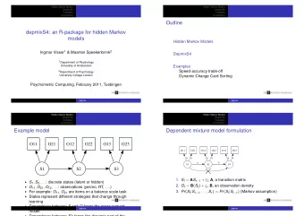
Markov Chains vs. HMMs When we have a 1 - 1 correspondence between alphabet letters and states, we have a Markov chain When such a correspondence does not hold, we only know the letters (observed data), and the states are “hidden”; hence, we have a hidden Markov model, or HMM
Markov Chains A C T G Associated with each edge is a transition probability
Markov Chains: The 1 - 1 Correspondence Sequence: GAGCGCGTAC S 1 :A S 2 :C S 3 :T S 4 :G States: S 4 S 1 S 4 S 2 S 4 S 2 S 4 S 3 S 1 S 2
HMMs: No 1 - 1 Correspondence (2 States Per Nucleotide) CpG states C + T + G + A + Non-CpG states G - A - T - C -
What’s Hidden? We can “ see” the nucleotide sequence We cannot see the sequence of states, or path, that generated the nucleotide sequence Hence, the state sequence (path) that generated the data is hidden
Markov Chains and HMMs In Markov chains and hidden Markov models, the probability of being in a state depends solely on the previous state Dependence on more than the previous state necessitates higher order Markov models
Sequence Annotation Using Markov Chains The annotation is straightforward: given the input sequence, we have a unique annotation (mapping between sequence letters and model states) The outcome is the probability of the sequence given the model
Sequence Annotation Using HMMs For every input sequence, there are many possible annotations (paths in the HMM) Annotation corresponds to finding the best mapping between sequence letters and model states (i.e., the path of highest probability that corresponds to the input sequence)
Markov Chains: Formal Definition A set Q of states Transition probabilities a st = P (x i =t|x i- 1 =s) : probability of state t given that the previous state was s In this model, the probability of sequence x=x 1 x 2 ...x L is L � P ( x ) = P ( x L | x L − 1 ) P ( x L − 1 | x L − 2 ) · · · P ( x 2 | x 1 ) P ( x 1 ) = P ( x 1 ) a x i − 1 x i i =2
Markov Chains: Formal Definition Usually, two states “ start” and “ end” are added to the Markov chain to model the beginning and end of sequences, respectively Adding these two states, the model defines a probability distribution on all possible sequences (of any length)
HMMs: Formal Definition A set Q of states An alphabet Σ Transition probability a st for every two states s and t Emission probability e k (b) for every letter b and state k (the probability of emitting letter b in state k)
HMMs: Sequences and Paths Due to the lack of a 1 - 1 correspondence, we need to distinguish between the sequence of letters (e.g., DNA sequences) and the sequence of states (path) For every sequence (of letters) there are many paths for generating it, each occurring with its probability We use x to denote a (DNA) sequence, and π to denote a (state) path
HMMs: The Model Probabilities Transition probability a k ℓ = P ( π i = ℓ | π i − 1 = k ) e k ( b ) = P ( x i = b | π i = k ) Emission probability
HMMs: The Sequence Probabilities The joint probability of an observed sequence and a path is L � P ( x, π ) = a 0 π 1 e π i ( x i ) a π i π i +1 i =1 The probability of a sequence is � P ( x ) = P ( x, π ) π
HMMs: The Parsing Problem Find the most probable state path that generates a given a sequence π ∗ = argmax π P ( x, π )
HMMs: The Posterior Decoding Problem Compute “ confidence” for the states on a path P ( π i = k | x )
HMMs: The Parameter Estimation Problem Compute the transition and emission probabilities of an HMM (from a given training data set)
A Toy Example: 5’ Splice Site Recognition From “What is a hidden Markov model?” , by Sean R. Eddy 5’ splice site indicates the “ switch” from an exon to an intron
A Toy Example: 5’ Splice Site Recognition Assumptions Uniform base composition on average in exons Introns are A/T rich (40% A/T, 10% G/C) The 5’ splice site consensus nucleotide is almost always a G (say, 95% G and 5% A)
A Toy Example: 5’ Splice Site Recognition
HMMs: A DP Algorithm for the Parsing Problem Let v k (i) denote the probability of the most probable path ending in state k with observation x i The DP structure: v ℓ ( i + 1) = e ℓ ( x i +1 ) max k ( v k ( i ) a k ℓ )
The Viterbi Algrorithm Initialization v 0 (0) = 1 , v k (0) = 0 ∀ k > 0 v � ( i ) = e � ( x i ) max k ( v k ( i − 1) a k � ) Recursion i = 1 . . . L ptr i ( � ) = argmax k ( v k ( i − 1) a k � ) P ( x, π ∗ ) = max k ( v k ( L ) a k 0 ) Termination L = argmax k ( v k ( L ) a k 0 ) π ∗ i − 1 = ptr i ( π ∗ i ) π ∗ Traceback i = 1 . . . L
The Viterbi Algrorithm Usually, the algorithm is implemented to work with logarithms of probabilities so that the multiplication turns into addition The algorithm takes O(Lq 2 ) time and O(Lq) space, where L is the sequence length and q is the number of states
A Toy Example: 5’ Splice Site Recognition
A Toy Example: 5’ Splice Site Recognition
Other Values of Interest The probability of a sequence, P (x) Posterior decoding: P ( π i = k | x ) Efficient DP algorithms for both using the forward and backward algorithms
The Forward Algorithm f k (i): the probability of the observed sequence up to and including x i , requiring that π i =k In other words, f k (i)= P (x 1 ,...,x i , π i =k) The structure of the DP algorithm: � f ℓ ( i + 1) = e ℓ ( x i +1 ) f k ( i ) a k ℓ k
The Forward Algorithm Initialization: f 0 (0) = 1 , f k (0) = 0 ∀ k > 0 � Recursion: f ℓ ( i ) = e ℓ ( x i ) f k ( i − 1) a k ℓ i = 1 . . . L k Termination: � P ( x ) = f k ( L ) a k 0 k
The Backward Algorithm b k (i): the probability of the last observed L-i letters, requiring that π i =k In other words, b k (i)= P (x L ,...,x i+1 | π i =k) The structure of the DP algorithm: � b ℓ ( i ) = a ℓ k e k ( x i +1 ) b k ( i + 1) k
The Backward Algorithm Initialization: b k ( L ) = a k 0 ∀ k � Recursion: b ℓ ( i ) = a ℓ k e ℓ ( x i +1 ) b k ( i + 1) i = L − 1 , . . . , 1 k Termination: � P ( x ) = a 0 k e k ( x 1 ) b k (1) k
The Posterior Probability f k ( i ) b k ( i ) = P ( x, π i = k ) = P ( π i = k | x ) P ( x ) ⇒ P ( π i = k | x ) = f k ( i ) b k ( i ) P ( x )
The Probability of a Sequence � P ( x ) = f k ( L ) a k 0 k � P ( x ) = a 0 k e k ( x 1 ) b k (1) k
Computational Requirements of the Algorithms Each of the algorithms takes O(Lq 2 ) time and O(Lq) space, where L is the sequence length and q is the number of states
A Toy Example: 5’ Splice Site Recognition
A Toy Example: 5’ Splice Site Recognition
Applications of Posterior Decoding (1) π ′ Find the sequence of states where π ′ i = argmax k P ( π i = k | x ) This is a more appropriate path when we are interested in the state assignment at a particular point i (however, this sequence of states may not be a legitimate path!)
Applications of Posterior Decoding (2) Assume function g(k) is defined on the set of states We can consider � G ( i | x ) = P ( π i = k | x ) g ( k ) k For example, for the CpG island problem, setting g(k)=1 for the “+” states, and g(k)=0 for the “-” states, G(i|x) is precisely the posterior probability according to the model that base i is in a CpG island
Recommend
More recommend
Explore More Topics
Stay informed with curated content and fresh updates.
