Lecture 9 Continuous-time Markov chains Dr. Dave Parker - PowerPoint PPT Presentation

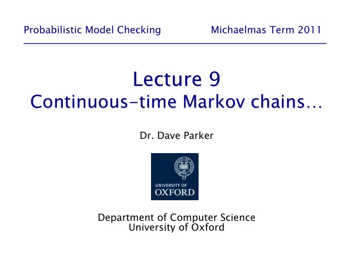
Probabilistic Model Checking Michaelmas Term 2011 Lecture 9 
 Continuous-time Markov chains… Dr. Dave Parker Department of Computer Science University of Oxford

Overview • Transient probabilities − uniformisation • Steady-state probabilities • CSL: Continuous Stochastic Logic − syntax − semantics − examples DP/Probabilistic Model Checking, Michaelmas 2011 2

Recall • Continuous-time Markov chain: C = (S,s init ,R,L) − R : S × S → ℝ ≥ 0 is the transition rate matrix − rates interpreted as parameters of exponential distributions • Embedded DTMC: emb(C)=(S,s init ,P emb(C) ,L) R (s, s' )/E(s) if E (s) 0 ⎧ > ⎪ P (s, s' ) 1 if E(s) 0 and s s' emb(C) = = = ⎨ 0 otherwise ⎪ ⎩ • Infinitesimal generator matrix R ( s , s ' ) s s ' ⎧ ≠ Q ( s , s ' ) = ∑ ≠ R ( s , s ' ) otherwise ⎨ − ⎩ s s ' DP/Probabilistic Model Checking, Michaelmas 2011 3

Transient and steady-state behaviour • Transient behaviour − state of the model at a particular time instant − π C s,t (s’) is probability of, having started in state s, being in state s’ at time t (in CTMC C) − π C (s’) = Pr s { ω ∈ Path C (s) | ω @t=s’ } s,t • Steady-state behaviour − state of the model in the long-run − π C s (s’) is probability of, having started in state s, being in state s’ in the long run − π C s (s’) = lim t →∞ π C s,t (s’) − intuitively: long-run percentage of time spent in each state DP/Probabilistic Model Checking, Michaelmas 2011 4

Computing transient probabilities • Consider a simple example − and compare to the case for DTMCs • What is the probability of being in state s 0 at time t? • DTMC/CTMC: 1 s 0 s 1 1 DP/Probabilistic Model Checking, Michaelmas 2011 5

Computing transient probabilities • Π t - matrix of transient probabilities − Π t (s,s’)= π s,t (s’) • Π t solution of the differential equation: Π t ’ = Π t · Q Q − where Q is the infinitesimal generator matrix • Can be expressed as a matrix exponential and therefore evaluated as a power series Π e ( Q t ) / i ! Q t i ∞ ⋅ ∑ = = ⋅ t i 0 = − computation potentially unstable − probabilities instead computed using uniformisation DP/Probabilistic Model Checking, Michaelmas 2011 6

Uniformisation • We build the uniformised DTMC unif(C) of CTMC C • If C =(S,s init ,R,L), then unif(C) = (S,s init ,P unif(C) ,L) − set of states, initial state and labelling the same as C − P unif(C) = I + Q/q − I is the |S| × |S| identity matrix − q ≥ max { E(s) | s ∈ S } is the uniformisation rate • Each time step (epoch) of uniformised DTMC corresponds to one exponentially distributed delay with rate q − if E(s)=q transitions the same as embedded DTMC (residence time has the same distribution as one epoch) − if E(s)<q add self loop with probability 1-E(s)/q (residence time longer than 1/q so one epoch may not be ‘long enough’) DP/Probabilistic Model Checking, Michaelmas 2011 7

Uniformisation - Example • CTMC C: 3 0 3 3 3 − R ⎡ ⎤ Q ⎡ ⎤ s 0 s 1 = = 2 0 2 2 − ⎢ ⎥ ⎢ ⎥ ⎣ ⎦ ⎣ ⎦ 2 • Uniformised DTMC unif(C) − let uniformisation rate q = max s { E(s) } = 3 1 1 0 1 1 0 − ⎡ ⎤ ⎡ ⎤ P unif ( C ) I Q / q ⎡ ⎤ = + = + = 0 1 2 2 2 1 − ⎢ ⎥ ⎢ ⎥ ⎢ ⎥ ⎣ ⎦ 3 ⎣ ⎦ ⎣ ⎦ 3 3 3 1 s 0 s 1 2/3 1/3 DP/Probabilistic Model Checking, Michaelmas 2011 8

Uniformisation • Using the uniformised DTMC the transient probabilities can be expressed by: unif ( C ) unif ( C ) Π e Q t e q ( P I ) t e ( q t ) P e q t ⋅ ⋅ − ⋅ ⋅ ⋅ − ⋅ = = = ⋅ t ( ) i i ( ) e ( q t ) P q t unif ( C ) ∞ − ⋅ ⋅ ∑ = ⋅ ⋅ i ! i 0 = ( ) ( i i ) e q t ( q t ) P unif ( C ) ∞ − ⋅ ⋅ ∑ = ⋅ ⋅ i ! i 0 = i ( ) γ P unif ( C ) ∞ ∑ = ⋅ q t , i i 0 ⋅ = P unif(C) is stochastic (all entries in [0,1] & rows sum to 1); ith Poisson probability with therefore computations with P are parameter q·t more numerically stable than Q DP/Probabilistic Model Checking, Michaelmas 2011 9

Uniformisation i ( ) Π γ P unif ( C ) ∞ ∑ = ⋅ ⋅ t q t , i i 0 = • (P unif(C) ) i is probability of jumping between each pair of states in i steps • γ q·t,i is the ith Poisson probability with parameter q·t − the probability of i steps occurring in time t, given each has delay exponentially distributed with rate q • Can truncate the (infinite) summation using the techniques of Fox and Glynn [FG88], which allow efficient computation of the Poisson probabilities DP/Probabilistic Model Checking, Michaelmas 2011 10

Uniformisation • Computing π s,t for a fixed state s and time t − can be computed efficiently using matrix-vector operations − pre-multiply the matrix Π t by the initial distribution − in this case: π s,0 (s’) equals 1 if s=s’ and 0 otherwise i π π Π ( ) π γ P unif ( C ) ∞ ∑ = ⋅ = ⋅ ⋅ s , t s , 0 t s , 0 q t , i i 0 ⋅ = i ( ) γ π P unif ( C ) ∞ ∑ = ⋅ ⋅ q t , i s , 0 i 0 ⋅ = − compute iteratively to avoid the computation of matrix powers i 1 i ( ) ( ) π P π P P unif ( C ) + unif ( C ) unif ( C ) ⋅ = ⋅ ⋅ s, t s, t DP/Probabilistic Model Checking, Michaelmas 2011 11

Uniformisation - Example • CTMC C, uniformised DTMC for q=3 3 0 3 3 3 0 1 − R ⎡ ⎤ Q ⎡ ⎤ ⎡ ⎤ s 0 s 1 P unif ( C ) = = = 2 0 2 2 2 1 − ⎢ ⎥ ⎢ ⎥ ⎢ ⎥ ⎣ ⎦ ⎣ ⎦ ⎣ ⎦ 3 3 2 • Initial distribution: π s0,0 = [ 1, 0 ] • Transient probabilities for time t = 1: i ( ) π γ π P unif ( C ) ∞ ∑ = ⋅ ⋅ s 0 , 1 q t , i s 0 , 0 i 0 ⋅ = 2 0 1 0 1 1 0 ⎡ ⎤ ⎡ ⎤ γ [ 1 , 0 ] ⎡ ⎤ γ [ 1 , 0 ] γ [ 1 , 0 ] ... = ⋅ ⋅ + ⋅ ⋅ + ⋅ ⋅ + 0 1 3 , 0 3 , 1 3 , 2 2 1 2 1 ⎢ ⎥ ⎢ ⎥ ⎢ ⎥ ⎣ ⎦ ⎣ ⎦ ⎣ ⎦ 3 3 3 3 ≈ [ 0.404043, 0.595957 ] DP/Probabilistic Model Checking, Michaelmas 2011 12

Steady-state probabilities • Limit π C s (s ’ ) = lim t →∞ π C s,t (s ’ ) − exists for all finite CTMCs − (see next slide) • As for DTMCs, need to consider the underlying graph structure of the Markov chain: − reachability (between pairs) of states − bottom strongly connected components (BSCCs) − one special case to consider: absorbing states are BSCCs − note: can do this equivalently on embedded DTMC • CTMC is irreducible if all its states belong to a single BSCC; otherwise reducible DP/Probabilistic Model Checking, Michaelmas 2011 13

Periodicity • Unlike for DTMCs, do not need to consider periodicity • e.g. probability of being in state s 0 at time t? • DTMC/CTMC: 1 s 0 s 1 1 DP/Probabilistic Model Checking, Michaelmas 2011 14

Irreducible CTMCs • For an irreducible CTMC: − the steady-state probabilities are independent of the starting state: denote the steady state probabilities by π C (s’) • These probabilities can be computed as − the unique solution of the linear equation system: C C π Q 0 and π ( s ) 1 ∑ ∈ ⋅ = = s S where Q is the infinitesimal generator matrix of C • Solved by standard means: − direct methods, such as Gaussian elimination − iterative methods, such as Jacobi and Gauss-Seidel DP/Probabilistic Model Checking, Michaelmas 2011 15

Balance equations C C π Q 0 and π ( s ) 1 ∑ ∈ ⋅ = = s S balance the rate of leaving and entering normalisation a state For all s ∈ S: π C (s) · (- Σ s ’ ≠ s R(s,s ’ )) + Σ s ’ ≠ s π C (s ’ ) · R(s ’ ,s) = 0 ⇔ π C (s) · Σ s ’ ≠ s R(s,s ’ ) = Σ s ’ ≠ s π C (s ’ ) · R(s ’ ,s) DP/Probabilistic Model Checking, Michaelmas 2011 16

Steady-state - Example • Solve: π ·Q=0 and ∑ π (s)=1 3 / 2 3 / 2 0 0 3/2 3/2 3/2 − ⎡ ⎤ {empty} {full} ⎢ ⎥ 3 9 / 2 3 / 2 0 − Q s 0 s 1 ⎢ ⎥ s 2 s 3 = 1 0 3 9 / 2 3 / 2 ⎢ ⎥ − ⎢ ⎥ 0 0 3 3 − 3 3 3 ⎣ ⎦ 3 / 2 π ( s ) 3 π ( s ) 0 − ⋅ + ⋅ = 0 1 3 / 2 π ( s ) 9 / 2 π ( s ) 3 π ( s ) 0 ⋅ − ⋅ + ⋅ = 0 1 2 3 / 2 π ( s ) 9 / 2 π ( s ) 3 π ( s ) 0 ⋅ − ⋅ + ⋅ = 1 2 3 3 / 2 π ( s ) 3 π ( s ) 0 ⋅ − ⋅ = 2 3 π ( s ) π ( s ) π ( s ) π ( s ) 1 + + + = 0 1 2 3 π = [ 8/15, 4/15, 2/15, 1/15 ] DP/Probabilistic Model Checking, Michaelmas 2011 17