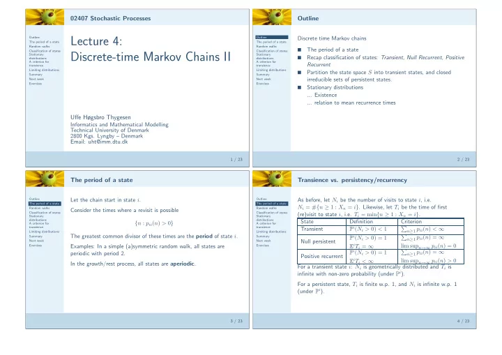
Lecture 4: Outline The period of a state The period of a state - - PowerPoint PPT Presentation

02407 Stochastic Processes

Outline The period of a state Random walks Classification of states Stationary distributions A criterion for transience Limiting distributions Summary Next week Exercises

1 / 23

Lecture 4: Discrete-time Markov Chains II

Uffe Høgsbro Thygesen

Informatics and Mathematical Modelling Technical University of Denmark 2800 Kgs. Lyngby – Denmark Email: uht@imm.dtu.dk

Outline

Outline The period of a state Random walks Classification of states Stationary distributions A criterion for transience Limiting distributions Summary Next week Exercises

2 / 23

Discrete time Markov chains

■

The period of a state

■

Recap classification of states: Transient, Null Recurrent, Positive Recurrent

■

Partition the state space S into transient states, and closed irreducible sets of persistent states.

■

Stationary distributions ... Existence ... relation to mean recurrence times

The period of a state

Outline The period of a state Random walks Classification of states Stationary distributions A criterion for transience Limiting distributions Summary Next week Exercises

3 / 23

Let the chain start in state i. Consider the times where a revisit is possible {n : pii(n) > 0} The greatest common divisor of these times are the period of state i. Examples: In a simple (a)symmetric random walk, all states are periodic with period 2. In the growth/rest process, all states are aperiodic.

Transience vs. persistency/recurrency

Outline The period of a state Random walks Classification of states Stationary distributions A criterion for transience Limiting distributions Summary Next week Exercises

4 / 23

As before, let Ni be the number of visits to state i, i.e. Ni = #{n ≥ 1 : Xn = i}. Likewise, let Ti be the time of first (re)visit to state i, i.e. Ti = min{n ≥ 1 : Xn = i}. State Definition Criterion Transient Pi(Ni > 0) < 1

• n≥1 pii(n) < ∞

Null persistent Pi(Ni > 0) = 1 EiTi = ∞

• n≥1 pii(n) = ∞

lim supn→∞ pii(n) = 0 Positive recurrent Pi(Ni > 0) = 1 EiTi < ∞

• n≥1 pii(n) = ∞

lim supn→∞ pii(n) > 0 For a transient state i: Ni is geometrically distributed and Ti is infinite with non-zero probability (under Pi). For a persistent state, Ti is finite w.p. 1, and Ni is infinite w.p. 1 (under Pi).

State classification in general random walk

Outline The period of a state Random walks Classification of states Stationary distributions A criterion for transience Limiting distributions Summary Next week Exercises

5 / 23

Sn+1 = Sn + Xn , S0 = 0 where Xn are i.i.d. with mean µ and variance σ2. According to the Central Limit Theorem Sn

→

∼ N(nµ, nσ2) so p00(n) ≈ 1 √ 2πnσ2 exp

• −n

2 µ2 σ2

• Corollary (4) (p. 221) says that the state 0 is persistent iff
• n p00(n) = ∞. I.e., iff µ = 0.

Compare exercise 6.3.2 where we had Xn ∈ {−1, 2}.

Random walks in higher dimensions

Outline The period of a state Random walks Classification of states Stationary distributions A criterion for transience Limiting distributions Summary Next week Exercises

6 / 23

A vector process in N dimensions Xn = (X(1)

n , . . . , X(N) n

), where the co-ordinate processes X(i)

n

are independent biased random walks with mean µi and variance σ2

i .

p00(n) ≈ 1 (2πn)N/2 σi exp

• −n

2

• i

µ2

i

σ2

i

• The origin is null persistent iff ∀i : µi = 0 and n ≤ 2; otherwise

transient. (The conclusion can be generalized to the situation where the co-ordinate processes are correlated)

Connecting random walks and diffusion

Outline The period of a state Random walks Classification of states Stationary distributions A criterion for transience Limiting distributions Summary Next week Exercises

7 / 23

Compare the diffusion equation in C(x, t): ∂C ∂t = D∂2C ∂x2 with a symmetric random walk Sn with pi(i+1) = pi(i−1) = p, pii = 1 − 2p. 1. When n is large, Sn is approximately distributed as N(0, σ2n). Compare this with the solution of the diffusion equation with initial condition C(x, 0) = δ(x) C(x, t) = 1 √ 2π2Dt exp(−1 2 x2 2Dt) 2. Compare the forward equation for the random walk with the second-order central finite difference scheme for discretisation of the diffusion equation. (If you have studied numerics ...)

Survival analysis with competing hazards

Outline The period of a state Random walks Classification of states Stationary distributions A criterion for transience Limiting distributions Summary Next week Exercises

8 / 23

A model of the course of university studies of a single student: Xn ∈ N ∪ {G} ∪ {A} where Xn = i means that the student is at his/her ith semester, Xn = G means graduated, Xn = A means studies abandoned without graduation. Transition probabilities: piG = gi piA = ai pi(i+1) = 1 − gi − ai We can divide the state space into three: The transient states N, the absorbing state G and the absorbing state A.

Classification of state space

Outline The period of a state Random walks Classification of states Stationary distributions A criterion for transience Limiting distributions Summary Next week Exercises

9 / 23

Classification of state space

Outline The period of a state Random walks Classification of states Stationary distributions A criterion for transience Limiting distributions Summary Next week Exercises

10 / 23

C1 C2 T C3

Communicating states

Outline The period of a state Random walks Classification of states Stationary distributions A criterion for transience Limiting distributions Summary Next week Exercises

11 / 23

State i communicates with j (written i → j), if pij(m) > 0 for some m. In terms of the graph: If there is a path from i to j. i and j intercommunicates (written i ↔ j) if i → j and j → i. (If there is a closed path containing both i and j). ↔ is an equivalence relation on state space S. Two intercommunicating states must have the same qualitative properties (theorem 2): Same period, same persistency.

Closed and irreducible subsets of state space

Outline The period of a state Random walks Classification of states Stationary distributions A criterion for transience Limiting distributions Summary Next week Exercises

12 / 23

A closed set C is one which can never be departed, once entered: pij = 0 for all i ∈ C and all j ∈ C. An irreducible set C is one in which all states intercommunicate. The Decomposition theorem says that state space can be partitioned into the transient states T and closed irreducible sets Ci: S = T ∪ C1 ∪ C2 ∪ · · · When studying long-time behaviour, we can concentrate on the cases S = T and S = C1.

Stationary distributions

Outline The period of a state Random walks Classification of states Stationary distributions A criterion for transience Limiting distributions Summary Next week Exercises

13 / 23

We had µn+1 = µnP A distribution π on S (such that πj ≥ 0 and

j πj = 1) is

stationary iff π = πP This is important: In many applications, we only care about stationary distributions.

The symmetric simple random walk

Outline The period of a state Random walks Classification of states Stationary distributions A criterion for transience Limiting distributions Summary Next week Exercises

14 / 23

The stationarity equation π = πP reads πj = 1 2(πj−1 + πj+1)

• n the interior. The general solution is

πj = aj + b 1. With two reflecting barriers, πj = b on the interior. 2. With no barriers, no distribution can live up to this. So what can we do with the solution πj = 1?

The asymmetric simple random walk

Outline The period of a state Random walks Classification of states Stationary distributions A criterion for transience Limiting distributions Summary Next week Exercises

15 / 23

The stationarity equation π = πP reads πj = πj−1p + πj+1q

• n the interior. The general solution is

πj = c · p q j + k With p < 1

2 and a lower reflecting barrier at 0, we find k = 0, and a

geometrically decaying stationary distribution π.

A queue application

Outline The period of a state Random walks Classification of states Stationary distributions A criterion for transience Limiting distributions Summary Next week Exercises

16 / 23

A single server handles customers one at a time. There are two types of events: New customers arriving, and the completion of service of a customer. Sn models the queue length immediately after event no. n. When the queue is non-empty, the next event is either a new customer arriving (with probability p) or a customer departing (w.p. q = 1 − p). Result: A stationary queue length distribution exists iff the mean service time is smaller than the mean interarrival time. If the two times are equal, then Sn is null recurrent. If the mean service time is the greater, then all states are transient. The queue length grows to infinity.

Theorem 3: Existence of stationary distributions

Outline The period of a state Random walks Classification of states Stationary distributions A criterion for transience Limiting distributions Summary Next week Exercises

17 / 23

An irreducible chain has a stationary distribution π iff all states are positive recurrent. In this case, π is unique and is given by πi = 1 µi where µi is the mean recurrence time of i.

T=1 T=3 T=2

Theorem 6:

Outline The period of a state Random walks Classification of states Stationary distributions A criterion for transience Limiting distributions Summary Next week Exercises

18 / 23

If the chain is irreducible and persistent, there exists a unique (up to a multiplicative constant) positive root x of x = xP. The chain is non-null iff

i xi < ∞.

Examples: 1. The unrestricted simple random walk: xi = 1 for all i. The chain is null persistent. 2. Any irreducible chain on a finite state space is non-null.

A criterion for transience

Outline The period of a state Random walks Classification of states Stationary distributions A criterion for transience Limiting distributions Summary Next week Exercises

19 / 23

According to theorem 3, if we can find a stationary distribution, then the chain is positive recurrent. Theorem (10): Fix an arbitrary target state s ∈ S. The chain is transient iff there exists a bounded non-zero solution to yi =

• j:j=s

pijyj, i = s. The candidate solution is yi = P(the chain never visits state s|X0 = i) To verify this solution, condition on first transition.

Limiting distributions

Outline The period of a state Random walks Classification of states Stationary distributions A criterion for transience Limiting distributions Summary Next week Exercises

20 / 23

Theorem (17): For an irreducible aperiodic chain pij(n) → 1 µj as n → ∞ In the transient or null persistent case, µj = ∞ so pij(n) → 0. In the non-null persistent case, pij(n) → πj, the stationary distribution. Note: The limit probability does not depend on initial state.

Summary

Outline The period of a state Random walks Classification of states Stationary distributions A criterion for transience Limiting distributions Summary Next week Exercises

21 / 23

■

Partitioning of state space ... allows us to assume irreducibility

■

We have defined stationary distributions ... shown that the transition probalities converge to the stationary distribution in the long time ... related the stationary distribution to mean recurrence times ... and given criteria for when the stationary distribution exists

Next week

Outline The period of a state Random walks Classification of states Stationary distributions A criterion for transience Limiting distributions Summary Next week Exercises

22 / 23

Section 6.5 on time reversible processes Section 6.6 on finite state spaces. Section 6.8 on Birth and Poisson processes (if we have time).

Exercises

Outline The period of a state Random walks Classification of states Stationary distributions A criterion for transience Limiting distributions Summary Next week Exercises

23 / 23

Problem 3.12 from Wolff. Exercise uht-01. Exercise 6.4.8 from G & S. Hint: Do not find the stationary distribution by solving the equation π = πP. Rather use the properties of Poisson distributions. Exercise 6.3.1 from G & S. Hint: Use material from section 6.4 rather than 6.3. Assume r < 1, a0 < 1. Start by focusing on the state 0.