Identification by Laplace Transform in Nonlinear Panel or Time - PowerPoint PPT Presentation

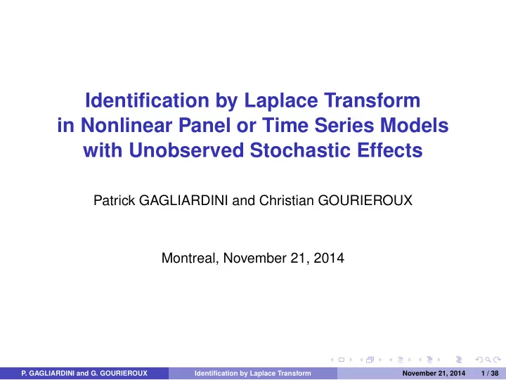
Identification by Laplace Transform in Nonlinear Panel or Time Series Models with Unobserved Stochastic Effects Patrick GAGLIARDINI and Christian GOURIEROUX Montreal, November 21, 2014 P. GAGLIARDINI and G. GOURIEROUX Identification by Laplace Transform November 21, 2014 1 / 38

1. INTRODUCTION This paper is about... ... identification in a general class of (semi-)parametric nonlinear models for time series or panel data with unobserved dynamic effects These models are characterized by an exponential affine specification for the nonlinear regression of data on lagged endogenous variables and unobserved dynamic effects P. GAGLIARDINI and G. GOURIEROUX Identification by Laplace Transform November 21, 2014 2 / 38

1. INTRODUCTION Exponential affine specifications are implied by standard distributional assumptions and are popular in asset pricing because of their analytical tractability The unobservable dynamic components capture time effects in panel data, stochastic volatilities and covolatilities of asset returns, systematic factors in risk analysis, etc. They complicate identification and estimation by standard methods such as Maximum Likelihood (ML) P. GAGLIARDINI and G. GOURIEROUX Identification by Laplace Transform November 21, 2014 3 / 38

1. INTRODUCTION The goal of the paper is to ... ... provide general procedures to obtain continuum sets of nonlinear moment restrictions for affine specifications based on the (conditional) Laplace transform Study when these sets of moment restrictions identify the nonlinear regression parameters, and the parametric or nonparametric specification for the distribution of dynamic effects The identification strategy naturally leads to Generalized Method of Moments (GMM) estimation P. GAGLIARDINI and G. GOURIEROUX Identification by Laplace Transform November 21, 2014 4 / 38

OUTLINE Introduction 1 The model: Examples and general specification 2 First-order moment restrictions: Nonlinear cross-differencing, moment 3 restrictions from Laplace transform Higher-order nonlinear moment restrictions 4 Application to linear and nonlinear latent factor models 5 P. GAGLIARDINI and G. GOURIEROUX Identification by Laplace Transform November 21, 2014 5 / 38

2. THE MODEL 2.1 Examples Example 1: Count panel data with stochastic time effect A Poisson dynamic panel regression model: i = 1 , ..., n , t = 1 , ..., T , ( n and T large ) y i , t ∼ P ( f t + α x i , t + cy i , t − 1 ) , with unobserved stochastic time effect f t Observed individual heterogeneity in the basic specification Extension to individual dynamic effects f i , t , e.g. “effort” processes for moral hazard in car insurance [Gourieroux, Jasiak (2004)] P. GAGLIARDINI and G. GOURIEROUX Identification by Laplace Transform November 21, 2014 6 / 38

2. THE MODEL 2.1 Examples Example 2: Linear factor model with lagged endogenous variables The vector y t of index returns for n markets t = 1 , ..., T y t = Bf t + Cy t − 1 + ε t , ( T large ) where the idiosyncratic shocks are ε t ∼ IIN ( 0 , Σ) and matrix Σ is diagonal The vector f t of K latent common factors represents systematic risks [see e.g. the Arbitrage Pricing Theory (APT), Ross (1976), Chamberlain, Rothschild (1983)] Lagged returns vector y t − 1 accounts for contagion (e.g. spillover) effects across markets P. GAGLIARDINI and G. GOURIEROUX Identification by Laplace Transform November 21, 2014 7 / 38

2. THE MODEL 2.1 Examples Example 3: Systematic risk and contagion in time series count data Multivariate time series count data y t = ( y 1 , t , ..., y m , t ) ′ Application to hedge fund survival: data are monthly liquidation counts in m management styles [Darolles, Gagliardini, Gourieroux (2011)] Conditionally on past counts and common factor path: j = 1 , ..., m , t = 1 , ..., T , ( T large ) y j , t ∼ P ( a j + b ′ j f t + c ′ j y t − 1 ) , Systematic risk factor f t with loading matrix B = [ b 1 , ..., b m ] ′ Contagion effects within and between groups through lagged counts and coefficients matrix C = [ c 1 , ..., c m ] ′ P. GAGLIARDINI and G. GOURIEROUX Identification by Laplace Transform November 21, 2014 8 / 38

2. THE MODEL 2.1 Examples Example 4: Conditionally Gaussian factor model with stochastic volatility in the factor y t = β h 1 / 2 t = 1 , ..., T ( T large ) η t + ε t , t with ( n , 1 ) loading vector β and bivariate latent factor f t = ( h t , η t ) ′ The factor stochastic volatility process ( h t ) , the common shock η t ∼ IIN ( 0 , 1 ) and the idiosyncratic shocks vector ε t ∼ IIN ( 0 , Σ) are mutually independent Process ( h t ) is an Autoregressive Gamma (ARG) Markov process with noncentral gamma transition: ρ u � � E [ exp ( uh t ) | h t − 1 ] = exp 1 − cuh t − 1 − δ log ( 1 − cu ) , where δ > 0 is the degree of freedom parameter, c > 0 is a scale parameter, and ρ ∈ ( 0 , 1 ) is the first-order autocorrelation P. GAGLIARDINI and G. GOURIEROUX Identification by Laplace Transform November 21, 2014 9 / 38

2. THE MODEL 2.1 Examples Example 5: Multivariate stochastic volatility model Vector of returns y t for n assets Tr ( B 1 Σ t )    + Σ 1 / 2 . t = 1 , ..., T y t = a + ( T large ) . ε t ,   t .  Tr ( B n Σ t ) where ε t ∼ IIN ( 0 , Id n ) Stochastic process Σ t of symmetric positive-definite ( n , n ) volatility-covolatility matrices: assume autoregressive Wishart dynamics [Bru (1991), Gourieroux (2006), Gourieroux, Jasiak, Sufana (2009)] Volatility risk premia parametrized by symmetric matrices B 1 , ..., B n See Gagliardini, Gourieroux (2014) for identification and estimation P. GAGLIARDINI and G. GOURIEROUX Identification by Laplace Transform November 21, 2014 10 / 38

2. THE MODEL 2.2 General specification Endogenous variable y t , with dimension n Unobservable dynamic effect f t , with dimension K Observable covariate process x t Information sets: let y t − 1 = ( y t − 1 , y t − 2 , ... ) and similarly for f t and x t Assumption A.1: Exponentially affine nonlinear regression model E [ exp ( u ′ y t ) | y t − 1 , f t , x t ] = exp a ( u , x t , θ ) ′ [ Bf t + Cy t − 1 + d ( x t , θ )] + b ( u , x t , θ ) � � where u is the multidimensional argument of the Laplace transform, θ , B , C are parameters (possibly constrained) and a , b , d are known functions. P. GAGLIARDINI and G. GOURIEROUX Identification by Laplace Transform November 21, 2014 11 / 38

2. THE MODEL 2.2 General specification Assumption A.2: Exogeneity, strict stationarity and Markov property of unobservable dynamic effects and observable regressors t ) ′ is: The joint process ( f ′ t , x ′ t ) ′ given i) exogenous and Markov, that is, the conditional distribution of ( f ′ t , x ′ y t − 1 , f t − 1 and x t − 1 depends on f t − 1 , x t − 1 only; ii) strictly stationary. The dynamics of the unobservable dynamic effect can be either specified parametrically, or let nonparametric P. GAGLIARDINI and G. GOURIEROUX Identification by Laplace Transform November 21, 2014 12 / 38

2. THE MODEL 2.2 General specification Nonlinear (semi-)affine state space specification as in Bates (2006), but suitable for the analysis of multivariate cross-sectional measurements (potentially of large dimension) The identification conditions in our moment-based setting are different from those in the likelihood-based framework of Bates (2006) The moment restrictions in this paper also differ from those underlying simulation based methods such as Simulated Method of Moments [SMM, McFadden (1989), Pakes, Pollard (1989)], Simulated Nonparametric Moments [SNM, Creel, Kristensen (2012)], etc. The (semi-)affine and (semi-)parametric framework in Assumption A.1 is more structural than the nonparametric setting in Hu, Shum (2012), Hu, Shiu (2013), allowing for more informative identifying restrictions P. GAGLIARDINI and G. GOURIEROUX Identification by Laplace Transform November 21, 2014 13 / 38

3. FIRST-ORDER NL MOMENT RESTRICTIONS 3.1 Nonlinear cross-differencing for panel data Assume that variables y i , t and f t are one-dimensional, and individual histories ( y i , t , x i , t ) , i varying, are independent conditional on factor path ( f t ) . Then: E [ exp ( uy i , t ) | y t − 1 , f t , x t ] = exp { a ( u , x i , t , θ )[ f t + cy i , t − 1 + d ( x i , t , θ )] + b ( u , x i , t , θ ) } i.e. � � exp { uy i , t − a ( u , x i , t , θ )[ cy i , t − 1 + d ( x i , t , θ )] − b ( u , x i , t , θ ) }| y t − 1 , f t , x t E exp [ a ( u , x i , t , θ ) f t ] , ∀ i , u , f t = (1) Assumption A.3*: The function u → a ( u , x i , t , θ ) is continuous and strictly monotonous w.r.t. argument u , for any given x i , t and θ. Then, we can define: u ( v , x i , t , θ ) as the solution of the equation a ( u , x i , t , θ ) = v , and replace argument u by u ( v , x i , t , θ ) in equation (1) P. GAGLIARDINI and G. GOURIEROUX Identification by Laplace Transform November 21, 2014 14 / 38