Lecture 21 Computational Methods for GPs Colin Rundel 04/10/2017 - PowerPoint PPT Presentation
Lecture 21 Computational Methods for GPs Colin Rundel 04/10/2017 1 GPs and Computational Complexity 2 + Chol () with (0, 1) 2 log || 1 2( ) 1 ( ) 2 log 2
Lecture 21 Computational Methods for GPs Colin Rundel 04/10/2017 1
GPs and Computational Complexity 2
𝝂 + Chol (𝚻) × 𝐚 with 𝑎 𝑗 ∼ 𝒪(0, 1) 2 log |Σ| − 1 2(𝐲 − 𝝂) ′ 𝚻 −1 (𝐲 − 𝝂) − 𝑜 2 log 2𝜌 {Σ} 𝑗𝑘 = 𝜏 2 exp (−{𝑒} 𝑗𝑘 𝜚) + 𝜏 2 𝑜 1 𝑗=𝑘 𝒫 (𝑜 2 ) Update covariance parameter? 𝒫 (𝑜 3 ) The problem with GPs Unless you are lucky (or clever), Gaussian process models are difficult to −1 Evaluate the (log) likelihood? 𝒫 (𝑜 3 ) Want to sample 𝐳 ? scale to large problems. For a Gaussian process 𝐳 ∼ 𝒪(𝝂, 𝚻) : 3
2 log |Σ| − 1 2(𝐲 − 𝝂) ′ 𝚻 −1 (𝐲 − 𝝂) − 𝑜 2 log 2𝜌 {Σ} 𝑗𝑘 = 𝜏 2 exp (−{𝑒} 𝑗𝑘 𝜚) + 𝜏 2 𝑜 1 𝑗=𝑘 𝒫 (𝑜 2 ) Update covariance parameter? 𝒫 (𝑜 3 ) The problem with GPs Unless you are lucky (or clever), Gaussian process models are difficult to −1 Evaluate the (log) likelihood? 𝒫 (𝑜 3 ) Want to sample 𝐳 ? scale to large problems. For a Gaussian process 𝐳 ∼ 𝒪(𝝂, 𝚻) : 3 𝝂 + Chol (𝚻) × 𝐚 with 𝑎 𝑗 ∼ 𝒪(0, 1)
{Σ} 𝑗𝑘 = 𝜏 2 exp (−{𝑒} 𝑗𝑘 𝜚) + 𝜏 2 𝑜 1 𝑗=𝑘 The problem with GPs Unless you are lucky (or clever), Gaussian process models are difficult to 𝒫 (𝑜 2 ) Update covariance parameter? 𝒫 (𝑜 3 ) 3 −1 Evaluate the (log) likelihood? 𝒫 (𝑜 3 ) Want to sample 𝐳 ? scale to large problems. For a Gaussian process 𝐳 ∼ 𝒪(𝝂, 𝚻) : 𝝂 + Chol (𝚻) × 𝐚 with 𝑎 𝑗 ∼ 𝒪(0, 1) 2 log |Σ| − 1 2(𝐲 − 𝝂) ′ 𝚻 −1 (𝐲 − 𝝂) − 𝑜 2 log 2𝜌
The problem with GPs −1 𝒫 (𝑜 2 ) Update covariance parameter? 𝒫 (𝑜 3 ) Unless you are lucky (or clever), Gaussian process models are difficult to 3 Evaluate the (log) likelihood? 𝒫 (𝑜 3 ) Want to sample 𝐳 ? scale to large problems. For a Gaussian process 𝐳 ∼ 𝒪(𝝂, 𝚻) : 𝝂 + Chol (𝚻) × 𝐚 with 𝑎 𝑗 ∼ 𝒪(0, 1) 2 log |Σ| − 1 2(𝐲 − 𝝂) ′ 𝚻 −1 (𝐲 − 𝝂) − 𝑜 2 log 2𝜌 {Σ} 𝑗𝑘 = 𝜏 2 exp (−{𝑒} 𝑗𝑘 𝜚) + 𝜏 2 𝑜 1 𝑗=𝑘
A simple guide to computational complexity 𝒫 (𝑜) - Linear complexity - Go for it 𝒫 (𝑜 2 ) - Quadratic complexity - Pray 𝒫 (𝑜 3 ) - Cubic complexity - Give up 4
A simple guide to computational complexity 𝒫 (𝑜) - Linear complexity - Go for it 𝒫 (𝑜 2 ) - Quadratic complexity - Pray 𝒫 (𝑜 3 ) - Cubic complexity - Give up 4
A simple guide to computational complexity 𝒫 (𝑜) - Linear complexity - Go for it 𝒫 (𝑜 2 ) - Quadratic complexity - Pray 𝒫 (𝑜 3 ) - Cubic complexity - Give up 4
A simple guide to computational complexity 𝒫 (𝑜) - Linear complexity - Go for it 𝒫 (𝑜 2 ) - Quadratic complexity - Pray 𝒫 (𝑜 3 ) - Cubic complexity - Give up 4
A simple guide to computational complexity 𝒫 (𝑜) - Linear complexity - Go for it 𝒫 (𝑜 2 ) - Quadratic complexity - Pray 𝒫 (𝑜 3 ) - Cubic complexity - Give up 4
A simple guide to computational complexity 𝒫 (𝑜) - Linear complexity - Go for it 𝒫 (𝑜 2 ) - Quadratic complexity - Pray 𝒫 (𝑜 3 ) - Cubic complexity - Give up 4
How bad is the problem? 5 30 method 20 time (secs) chol inv LU inv QR inv 10 0 2500 5000 7500 10000 n
2. Calc. chol (Σ 𝑞 − Σ 𝑞𝑝 Σ −1 𝑝 Σ 𝑝𝑞 ) 3. Calc. 𝜈 𝑞|𝑝 + chol (Σ 𝑞|𝑝 ) × 𝑎 0.467 • CPU (28.9 min) Total run time for 1000 posterior predictive draws: 1.732 Total 0.129 4. Calc. Allele Prob 0.049 Practice - Migratory Model Prediction After fitting the GP need to sample from the posterior predictive distribution 1.080 1. Calc. Σ 𝑞 , Σ 𝑞𝑝 , Σ 𝑞 CPU (secs) Step at ∼ 3000 locations 6 𝐳 𝑞 ∼ 𝒪 (𝜈 𝑞 + Σ 𝑞𝑝 Σ −1 𝑝 (𝑧 𝑝 − 𝜈 𝑝 ), Σ 𝑞 − Σ 𝑞𝑝 Σ −1 𝑝 Σ 𝑝𝑞 )
Practice - Migratory Model Prediction After fitting the GP need to sample from the posterior predictive distribution • CPU (28.9 min) Total run time for 1000 posterior predictive draws: 1.732 Total 0.129 4. Calc. Allele Prob 0.049 0.467 6 1.080 1. Calc. Σ 𝑞 , Σ 𝑞𝑝 , Σ 𝑞 CPU (secs) Step at ∼ 3000 locations 𝐳 𝑞 ∼ 𝒪 (𝜈 𝑞 + Σ 𝑞𝑝 Σ −1 𝑝 (𝑧 𝑝 − 𝜈 𝑝 ), Σ 𝑞 − Σ 𝑞𝑝 Σ −1 𝑝 Σ 𝑝𝑞 ) 2. Calc. chol (Σ 𝑞 − Σ 𝑞𝑝 Σ −1 𝑝 Σ 𝑝𝑞 ) 3. Calc. 𝜈 𝑞|𝑝 + chol (Σ 𝑞|𝑝 ) × 𝑎
A bigger hammer? 0.052 • CPU+GPU (7.8 min) • CPU (28.9 min) Total run time for 1000 posterior predictive draws: 3.7 0.465 1.732 Total 1.0 0.127 0.129 4. Calc. Allele Prob 0.9 0.049 Step 2.3 0.208 0.467 23.0 0.046 1.080 1. Calc. Σ 𝑞 , Σ 𝑞𝑝 , Σ 𝑞 Rel. Perf CPU+GPU (secs) CPU (secs) 7 2. Calc. chol (Σ 𝑞 − Σ 𝑞𝑝 Σ −1 𝑝 Σ 𝑝𝑞 ) 3. Calc. 𝜈 𝑞|𝑝 + chol (Σ 𝑞|𝑝 ) × 𝑎
Cholesky CPU vs GPU (P100) 8 30 method chol inv LU inv 20 time (secs) QR inv comp cpu 10 gpu 0 2500 5000 7500 10000 n
9 10.0 method chol inv LU inv time (secs) QR inv comp cpu 0.1 gpu 2500 5000 7500 10000 n
Relative Performance 10 Relative performance 10 method chol inv LU inv QR inv 1 2500 5000 7500 10000 n
Aside (1) - Matrix Multiplication 11 Matrix Multiplication 7.5 time (sec) comp 5.0 cpu gpu 2.5 0.0 2500 5000 7500 10000 n
12 Matrix Multiplication − Relative Performance 45 40 35 time (sec) 30 25 20 2500 5000 7500 10000 n
Aside (2) - Memory Limitations A general covariance is a dense 𝑜 × 𝑜 matrix, meaning it will require 𝑜 2 × 13 64-bits to store. 20 15 Cov Martrix Size (GB) 10 5 0 0 10000 20000 30000 40000 50000 n
Other big hammers • Able to fit models on the order of 𝑜 = 65 k (32 GB Cov. matrix) bigGP is an R package written by Chris Paciorek (UC Berkeley), et al. 14 • Specialized distributed implementation of linear algebra operation for GPs • Uses both shared and distributed memory • Designed to run on large super computer clusters Cholesky Decomposition 1000 Execution time, seconds (log scale) 100 10 1 6 cores 0.1 60 cores 816 cores 12480 cores 49920 cores 0.01 2048 8192 32768 131072 Matrix dimension, n (log scale)
More scalable solutions? • Spectral domain / basis functions • Covariance tapering • GMRF approximations • Low-rank approximations • Nearest-neighbor models 15
Low Rank Approximations 16
𝑊 𝑢 𝑜×𝑜 diag ( ̃ 𝑜×𝑛 = 𝑉 𝑊 𝑢 diag ( ̃ = 𝑇) 𝑜×𝑛 𝑛×𝑛 Low rank approximations in general ̃ 𝑉 𝑇) 𝑙×𝑙 ̃ 𝑙×𝑛 𝑜×𝑙 𝑁 Lets look at the example of the singular value decomposition of a matrix, ̃ 𝑁 𝑜×𝑛 𝑛×𝑛 where 𝑉 are called the left singular vectors, 𝑊 the right singular vectors, and 𝑇 the singular values. Usually the singular values and vectors are ordered such that the singular values are in descending order. The Eckart–Young theorem states that we can construct an approximatation of 𝑁 with rank 𝑙 by setting ̃ 𝑇 to contain only the 𝑙 largest singular values and all other values set to zero. 17 𝑊 𝑢 𝑜×𝑛 = 𝑉 𝑜×𝑜 diag (𝑇)
Low rank approximations in general ̃ 𝑙×𝑛 ̃ 𝑙×𝑙 𝑇) 𝑜×𝑙 𝑉 ̃ = 𝑛×𝑛 𝑜×𝑛 𝑇) Lets look at the example of the singular value decomposition of a matrix, 𝑁 and all other values set to zero. ordered such that the singular values are in descending order. 𝑁 𝑜×𝑛 𝑛×𝑛 𝑇 to contain only the 𝑙 largest singular values and 𝑇 the singular values. Usually the singular values and vectors are where 𝑉 are called the left singular vectors, 𝑊 the right singular vectors, The Eckart–Young theorem states that we can construct an approximatation of 𝑁 with rank 𝑙 by setting ̃ 17 𝑊 𝑢 𝑜×𝑛 = 𝑉 𝑜×𝑜 diag (𝑇) 𝑊 𝑢 𝑜×𝑜 diag ( ̃ 𝑜×𝑛 = 𝑉 𝑊 𝑢 diag ( ̃
Example ⎞ 0.58 −0.25 −0.32 −0.45 0.17) (−0.79 0.00 0.00 (1.50 ⎠ ⎟ ⎟ ⎟ −0.51 −0.51 −0.25 −0.51 −0.32 −0.37 −0.45 0.58 −0.79 ⎝ ⎜ ⎜ ⎜ ⎛ −0.37 −0.51) ̃ 0.333 ⎠ ⎟ ⎟ ⎟ ⎞ 0.140 0.166 0.203 0.249 0.166 0.200 0.251 0.203 = 0.251 0.330 0.501 0.249 0.333 0.501 1.000 ⎝ ⎜ ⎜ ⎜ ⎛ 𝑁 = Rank 2 approximation: 𝑁 = 0.333 ⎠ ⎟ ⎟ ⎟ ⎞ 0.143 0.167 0.200 0.250 0.167 0.200 0.250 0.200 0.00) 0.250 0.333 0.500 0.250 0.333 0.500 1.000 ⎝ ⎜ ⎜ ⎜ ⎛ 𝑉 = 𝑊 = ⎛ ⎜ −0.79 0.01 0.17 𝑇 = (1.50 ⎠ ⎟ ⎟ ⎟ ⎞ 0.51 −0.64 −0.51 −0.25 −0.10 ⎜ −0.51 −0.32 0.33 0.74 −0.37 −0.45 −0.03 −0.18 0.58 −0.79 ⎝ ⎜ 18 = 𝑉 diag (𝑇) 𝑊 𝑢
Recommend
More recommend
Explore More Topics
Stay informed with curated content and fresh updates.

