Lecture 1 Matthieu Bloch 1 Notation and basic definitions integers - PDF document

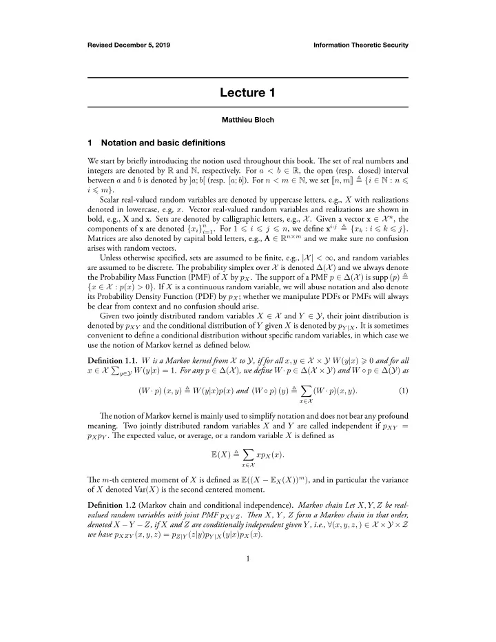
1 arises with random vectors. Tie notion of Markov kernel is mainly used to simplify notation and does not bear any profound (1) use the notion of Markov kernel as defined below. convenient to define a conditional distribution without specific random variables, in which case we We start by briefly introducing the notion used throughout this book. Tie set of real numbers and be clear from context and no confusion should arise. Revised December 5, 2019 Information Theoretic Security Lecture 1 Matthieu Bloch 1 Notation and basic definitions integers are denoted by R and N , respectively. For a < b ∈ R , the open (resp. closed) interval between a and b is denoted by ] a ; b [ (resp. [ a ; b ] ). For n < m ∈ N , we set � n, m � ≜ { i ∈ N : n ⩽ i ⩽ m } . Scalar real-valued random variables are denoted by uppercase letters, e.g., X with realizations denoted in lowercase, e.g, x . Vector real-valued random variables and realizations are shown in bold, e.g., X and x . Sets are denoted by calligraphic letters, e.g., X . Given a vector x ∈ X n , the i =1 . For 1 ⩽ i ⩽ j ⩽ n , we define x i : j ≜ { x k : i ⩽ k ⩽ j } . components of x are denoted { x i } n Matrices are also denoted by capital bold letters, e.g., A ∈ R n × m and we make sure no confusion Unless otherwise specified, sets are assumed to be finite, e.g., |X| < ∞ , and random variables are assumed to be discrete. Tie probability simplex over X is denoted ∆( X ) and we always denote the Probability Mass Function (PMF) of X by p X . Tie support of a PMF p ∈ ∆( X ) is supp ( p ) ≜ { x ∈ X : p ( x ) > 0 } . If X is a continuous random variable, we will abuse notation and also denote its Probability Density Function (PDF) by p X ; whether we manipulate PDFs or PMFs will always Given two jointly distributed random variables X ∈ X and Y ∈ Y , their joint distribution is denoted by p XY and the conditional distribution of Y given X is denoted by p Y | X . It is sometimes Definition 1.1. W is a Markov kernel from X to Y , if for all x, y ∈ X × Y W ( y | x ) ⩾ 0 and for all x ∈ X � y ∈Y W ( y | x ) = 1 . For any p ∈ ∆( X ) , we define W · p ∈ ∆( X × Y ) and W ◦ p ∈ ∆( Y ) as � ( W · p ) ( x, y ) ≜ W ( y | x ) p ( x ) and ( W ◦ p ) ( y ) ≜ ( W · p )( x, y ) . x ∈X meaning. Two jointly distributed random variables X and Y are called independent if p XY = p X p Y . Tie expected value, or average, or a random variable X is defined as � E ( X ) ≜ xp X ( x ) . x ∈X Tie m -th centered moment of X is defined as E (( X − E X ( X )) m ) , and in particular the variance of X denoted Var ( X ) is the second centered moment. Definition 1.2 (Markov chain and conditional independence) . Markov chain Let X, Y, Z be real- valued random variables with joint PMF p XY Z . Tien X , Y , Z form a Markov chain in that order, denoted X − Y − Z , if X and Z are conditionally independent given Y , i.e., ∀ ( x, y, z, ) ∈ X ×Y ×Z we have p XZY ( x, y, z ) = p Z | Y ( z | y ) p Y | X ( y | x ) p X ( x ) .

2 Convexity plays a central role in many of our proofs, largely because information-theoretic metrics where we have used Jensen’s inequality. (3) Tien, generally for continuous random variables. log-sum inequality in subsequent chapters and we recall these results here for completeness. possess convenient convexity properties. We shall extensively use Jensen’s inequality and the related (2) Finally, we define the notion of absolute continuity that will prove useful in later sections. Revised December 5, 2019 Information Theoretic Security Definition 1.3 (Absolute continuity) . Let p, q ∈ ∆( X ) . We say that p is absolutely continuous with respect to (w.r.t.) q , denoted by p ≪ q , if supp ( p ) ⊆ supp ( q ) . If p is not absolutely continuous w.r.t. q , we write p ≪ / q . 2 Convexity and Jensen’s inequality Definition 2.1 (Convex and concave functions) . A function f : � a, b � �− → R is convex if ∀ λ ∈ � 0 , 1 � f ( λa + (1 − λ ) b ) ⩽ λf ( a ) + (1 − λ ) f ( b ) . A function f is strictly convex if the inequality above is strict. A function f is (strictly) concave if − f is (strictly) convex. Tieorem 2.2 (Jensen’s inequality) . Jensen’s inequality Let X be a real-valued random variable defined on some interval [ a, b ] and with PDF p X . Let f : [ a, b ] → R be a real valued function that is convex in [ a, b ] . Tien, f ( E ( X )) ⩽ E ( f ( X )) . For any strictly convex function, equality holds if and only if X is a constant. Tie results also holds more Proof. Let h L : [ a, b ] → R be a line such that ∀ x ∈ � a, b � h L ( x ) ⩽ f ( x ) . Such a line always exists as a result of convexity. Tien, E ( h L ( X )) ⩽ E ( f ( X )) , but since h L is a line, we have h L ( E ( X )) = E ( h L ( X )) ⩽ E ( f ( X )) . In particular, we can choose h L such that h L ( E ( X )) = f ( E ( X )) because f is convex. Hence, f ( E ( X )) ⩽ E ( f ( X )) and if f is strictly convex, we have equality if and only if X = cst. ■ Corollary 2.3 (Log-sum inequality) . log-sum inequality Let { a i } n i =1 ∈ R n + and { b i } n i =1 ∈ R n + . � n n � ln ( � n i =1 a i ) a i ln a i � � ⩾ a i i =1 b i ) . ( � n b i i =1 i =1 Proof. Note that if b j = 0 and a j � = 0 for some j ∈ � 1 , n � then the results holds since the left- hand-side of (2) is infinite. If not, we introduce the function f : R + → R : x �→ x ln x with the convention that f (0) = 0 , which is infinitely differentiable on its domain. Since f ′′ ( x ) = 1 ⩾ 0 , f is convex. Set a ≜ � n i =1 a i and b ≜ � n i =1 b i . Tien, note that � n n n n � � a i � a i ln a i b i a i a i � a = a ln a � � � � � ⩾ bf = = b = bf b i f b , b i b i b b i b b i =1 i =1 i =1 i =1 ■ Proposition 2.4. Let X be a real-valued random variable defined on some interval [ a, b ] and with PDF p X . Let f : [ a, b ] → R be a real valued function that is convex in [ a, b ] . Tien, E ( f ( X )) ⩽ f ( a ) + f ( b ) − f ( a ) ( E ( X ) − a ) b − a

3 As we will see in subsequent chapters, many information-theoretic security metrics can be expressed (12) interval (11) (10) (9) (8) (7) (6) (5) expressed more generally as shown in the next proposition. (4) is two distances, the total variation distance and the relative entropy, which we shall extensively use. in terms of how close or distinct probability distributions are. We develop here the properties of Revised December 5, 2019 Information Theoretic Security For any strictly convex function, the equality holds if and only if X is only distributed on the end of the Proof. Let h U : [ a, b ] → R be a line such that ∀ x ∈ � a, b � f ( x ) ⩽ h U ( x ) . Tien, E ( f ( X )) ⩽ E ( h U ( X )) = h U ( E ( X )) . In particular, we may choose h U : x �→ f ( a ) + f ( b ) − f ( a ) ( x − a ) . b − a Hence, E ( f ( X )) ⩽ f ( a ) + f ( b ) − f ( a ) ( E ( X ) − a ) and if f is strictly convex, equality holds if X is b − a such that p X ( x ) = 0 for x ∈ ] a, b [ . ■ 3 Distances between distributions Definition 3.1 (Total variation distance) . Tie total variation between two distributions p, q ∈ ∆( X ) V ( p, q ) ≜ 1 2 � p − q � 1 ≜ 1 � | p ( x ) − q ( x ) | . 2 x ∈X For all practical purposes, the total variation distance is an ℓ 1 norm on the probability simplex ∆( X ) and inherits all its properties (symmetry, positivity, triangle, inequality). Tie normalization by 1 2 is for convenience as we shall see from the properties derived next. Tie total variation can be Proposition 3.2. Tie total variation between two distributions p, q ∈ ∆( X ) is ( P p ( E ) − P q ( E )) = sup ( P q ( E ) − P p ( E )) . V ( p, q ) = sup E⊂X E⊂X Tie supremum is attained for E ≜ { x : ∈ X : p ( x ) > q ( x ) } . Consequently, 0 ⩽ V ( p, q ) ⩽ 1 . Proof. From the definition, upon setting E 0 ≜ { x ∈ X : p ( x ) > q ( x ) } we have V ( p, q ) = 1 ( p ( x ) − q ( x )) + 1 � � ( q ( x ) − p ( x )) 2 2 x : ∈E c x ∈E 0 0 = 1 2 ( P p ( E 0 ) − P q ( E 0 ) + P q ( E c 0 ) − P p ( E c 0 )) = P p ( E 0 ) − P q ( E 0 ) ⩽ sup ( P p ( E ) − P q ( E )) . E⊂X Conversely, note that for every E P p ( E ) − P q ( E ) = 1 2 ( P p ( E ) − P q ( E ) + P q ( E c ) − P p ( E c )) = 1 ( p ( x ) − q ( x )) + 1 � � ( q ( x ) − p ( x )) 2 2 x ∈E x : ∈E c ⩽ V ( p, q ) , so that sup E⊂X ( P p ( E ) − P q ( E )) ⩽ V ( p, q ) . ■