1 A statistical definition of probability: frequentist 2 concepts: - PDF document
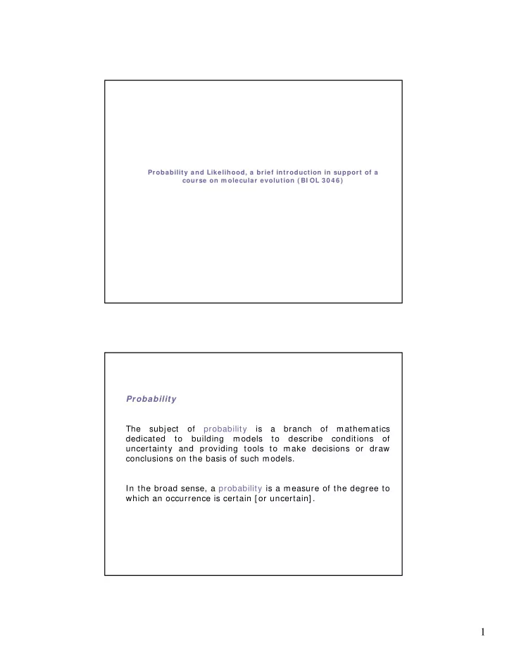
Probability and Likelihood, a brief introduction in support of a course on m olecular evolution ( BI OL 3 0 4 6 ) Probability The subject of probability is a branch of mathematics dedicated to building models to describe conditions of
Probability and Likelihood, a brief introduction in support of a course on m olecular evolution ( BI OL 3 0 4 6 ) Probability The subject of probability is a branch of mathematics dedicated to building models to describe conditions of uncertainty and providing tools to make decisions or draw conclusions on the basis of such models. In the broad sense, a probability is a measure of the degree to which an occurrence is certain [ or uncertain] . 1
A statistical definition of probability: frequentist 2 concepts: 1. Sam ple space , S , is the collection [ sometimes called universe] of all possible outcomes. The sample space is a set where each outcome comprises one element of the set. 2. Relative frequency is the proportion of the sample space on which an event E occurs. In an experiment with 100 outcomes, and E occurs 81 times, the relative frequency is 81/ 100 or 0.81. A statistical definition of probability: frequentist The statistical definition is derived from statistical regularity. Statistical regularity is the property of a relative frequency in the long run, over replicates, where the cumulative relative frequency (crf) of an event (E) stabilizes. The crf is simply the relative frequency computed cumulatively over some number of replicates of samples, each with a space S. 2
Month Number of Number Cum ulative S Cum ulative E crf subjects ( S) Controlled ( E) 1 100 80 100 80 0.800 2 100 88 200 168 0.840 3 100 75 300 243 0.810 4 100 77 400 320 0.800 5 100 80 500 400 0.800 6 100 76 600 476 0.793 7 100 82 700 558 0.797 8 100 79 800 637 0.796 9 100 80 900 717 0.797 10 100 76 1000 793 0.793 11 100 77 1100 970 0.791 12 100 78 1200 948 0.790 [ data for example is after McColl (1995)] In words, the probability of an event E, written as P(E), is the long run (cumulative) relative frequency of E. ( ) = P(E) lim E crf n → ∞ n ( ) = P(E) lim E crf n → ∞ n 1 0.9 0.8 0.7 0.6 0.5 0.4 0.3 0.2 0.1 0 0 2500 5000 7500 10000 Hypothetical plot of crf of an event 3
Probability axiom s: 1. Probability scale= 1 to 0. Hence, 0 ≤ P(E) ≤ 1. 2. Probabilities are derived from a relative frequency of an event (E) in the “space of all possible outcomes” ( S ), where P( S) = 1 . Hence, if the probability of an event (E) is P(E), then the probability that E does not occur is 1 – P(E). 3. When events E and F are disjoint , they cannot occur together. The probability of disjoint events E or F = P(E or F) = P(E) + P(F). 4. Axiom 3 above deals with a finite sequence of events. Axiom 4 is an extension of axiom 3 to an infinite sequence of events. Product rule: The product rule applies when two events E1 and E2 are independent . E1 and E2 are independent if the occurrence or non-occurrence of E1 does not change the probability of E2 [ and vice versa] . [ A further statistical definition requires the use of the multiplication theorem ] I t is important to note that a proof of statistical independence for a specific case by using the m ultiplication theorem is rarely possible; hence, most models incorporate independence as a model assumption. When E1 and E2 occur together they are joint events. The joint probability of the independent events E1 and E2 = P(E1,E2) = P(E1) × P(E2). Hence the term “product rule” or “multiplication principle”, or whatever you call it. 4
Conditional probability: is the probability of event E2 assuming that event E1 has already occurred. We assume the E1 and E2 events are in a given sample space, S, and P(E1) > 0. We write it as P(E2| E1); the vertical bar is read as “given”. Exam ple for “jog your m em ory”: Suppose we have two fair dice: For one: S = 1,2,3,4,5 & 6 P(S) = 1 P(1), ..., P(6) = 1/ 6, … , 1/ 6 For two: S = 36 different pairs of integers [ 1,6] You roll Die # 1; what is the probability that you roll a “5” or a “6”? Die 1: P(5) = 1/ 6 and P(6) = 1/ 6 P(5 or 6) = P(5) + P(6) = 1/ 3 You roll both dice: what is the probability that you roll two “5”s? P(5,5) = P(5) × P(5) = 1/ 6 × 1/ 6 = 1/ 36 5
Exam ple for “jog your m em ory”: What about the conditional probability that second roll is a “5” given the first was a “5”? We write this as follows: ( 1 , 2 ) P E E = ( 1 | 2 ) P E E ( 2 ) P E 1 ( 5 , 5 ) P 36 = P = = 1 ( 5 | 5 ) P 6 ( 5 ) 1 / 6 There is a logically satisfying result: since the two rolls are independent, it should not matter what the first roll was, and indeed the outcome of the second roll [ conditional on the first roll] was 1/ 6. Probability m odel ⎛ ⎞ n ( ) ( ) − = ⎜ ⎟ − k n k 1 P ⎜ ⎟ p p ⎝ ⎠ k ⎛ ⎞ n ! ⎜ ⎟ = n ( ) ⎜ ⎟ − ! ! k n k ⎝ ⎠ k Coin toss example: what is the probability of obtaining, say, 5 heads given a fair coin (p = 0.5) and 12 tosses? P(k= 5 | p= 0.5, n= 12). 6
Probability m odel ( ) = = = = 5 | 0 . 5 , 12 P k p n ⎛ ⎞ 12 ( ) ( ) − ⎟ = ⎜ × − 5 12 5 0 . 5 1 0 . 5 ⎜ ⎟ ⎝ 5 ⎠ ⎛ ⎞ 12 12 ! ⎜ ⎟ = ⎜ ⎟ ( ) ! − ⎝ 5 ⎠ 5 ! 12 5 Probability and likelihood are inverted Probability refers to the occurrence of some future outcome. • For example: “If I toss a fair coin 12 times, what is the probability that I will obtain 5 heads and 7 tails?” Likelihood refers to a past event with a known outcome. • For example: “What is the probability that my coin is fair if I tossed it 12 times and observed 5 heads and 7 tails ” 7
Case 1 : probability The question is the same: “If I toss a fair coin 12 times, what is the probability that I will obtain 5 heads and 7 tails?” The answer comes directly from the above formula where n = 12, and k = 5. The probability of such a future event is 0.193359. Probability of 5 heads & 7 tails = 0 .1 9 3 3 The curve is a normal approxim ation to the binomial distribution Our outcom e of 5 heads & 7 tails Axiom 2 : P( S) = 1 ; the probability of each outcom e ( i.e., 0 to 1 2 heads) sum to 1 . 8
Case 2 : likelihood The second question is: “What is the probability that my coin is fair if I tossed it 12 times and observed 5 heads and 7 tails?” We have inverted the problem: In case 1: we were interested in the probability of a future outcome given that my coin is fair. In case 2: we are interested in the probability that my coin is fair, given a particular outcome. So, in the likelihood framework we have inverted the question such that the hypothesis (H) is variable, and the outcome (let’s call it the data, D) is constant. We are interested in P(H| D), but we have a problem… Case 2 : likelihood A problem: What we want to measure is P(H| D). The problem is that we can’t work with the probability of a hypothesis, only the relative frequencies of outcomes. The solution: The P(H| D) = α P(D| H) The P(H| D) = α P(D| H) The P(H| D) = α P(D| H) Constant value of proportionality Constant value of proportionality Constant value of proportionality 9
⎛ ⎞ n ( ) ( ) − = ⎜ ⎟ − k n k 1 P ⎜ ⎟ p p ⎝ ⎠ k P ROBABI LI TI ES Data D1: 1H & 1T D2: 2H Hypotheses H1: p(H) = 1/ 4 0 .3 7 5 0 .0 6 2 5 H2: p(H) = 1/ 2 0 .5 0 .2 5 ⎛ ⎞ n ( ) ( ) − = ⎜ ⎟ − k n k 1 P ⎜ ⎟ p p ⎝ ⎠ k L I KELI HOODS Data D1: 1H & 1T D2: 2H α 1 × 0 .3 7 5 α 2 × 0 .0 6 2 5 Hypotheses H1: p(H) = 1/ 4 α 1 × 0 .5 α 2 × 0 .2 5 H2: p(H) = 1/ 2 H1 is less likely than H2 by a factor of ¾ . The fram ew ork here is one of relative support. 10
An exam ple of Likelihood in action Coin toss: What is likelihood that my coin is “fair” given 12 tosses with 5 heads and 7 tails? Is the hypothesis of “fairness” the best explanation of these data? The P(H| D) = α × P(D| H) L = α × P(D| H) L = P(D| H) ⎛ ⎞ n ( ) ( ) − = ⎜ ⎟ − k n k 1 P ⎜ ⎟ p p ⎝ ⎠ k D = outcome ( n choose k ) H = probability ( p ) Maxim um Likelihood score = 0 .2 2 8 0.25 p = 0 .5 ( L = 0 .1 9 3 ) 0.2 0.15 0.1 0.05 0 0 0.2 0.4 0.6 0.8 1 ML estim ate of p = 0 .4 2 Likelihood that the coin is fair (p = 0.5) is 0.193. This is less likely than the MLE by about 15% [ X; w rong in slides PDF ] 11
Don’t forget, the area under the likelihood curve does not sum to 1 How many have had a course in statistics? How many found this review useful? How many would like further review in statistics? 12
Recommend
More recommend
Explore More Topics
Stay informed with curated content and fresh updates.
