Contents of the Lecture Multiple random variables Covariance, - PowerPoint PPT Presentation

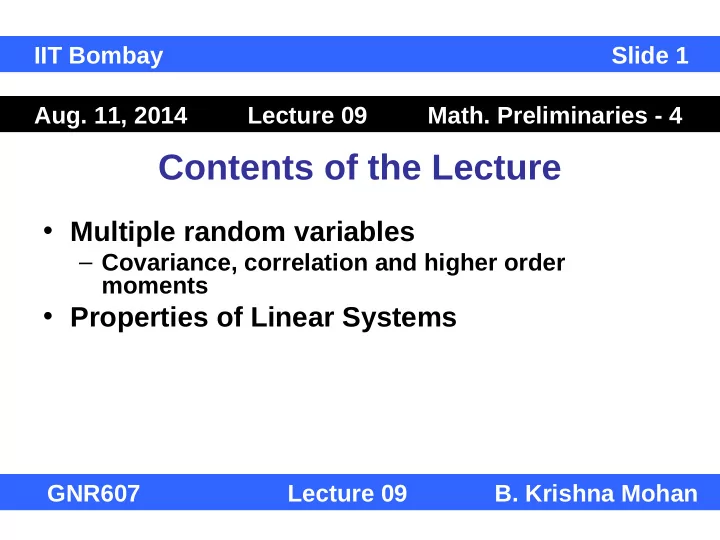
IIT Bombay Slide 1 Aug. 11, 2014 Lecture 09 Math. Preliminaries - 4 Contents of the Lecture • Multiple random variables – Covariance, correlation and higher order moments • Properties of Linear Systems GNR607 Lecture 09 B. Krishna Mohan

IIT Bombay Slide 2 Gaussian Distribution Source: http://allpsych.com/researchmethods/distributions.html GNR607 Lecture 09 B. Krishna Mohan

IIT Bombay Slide 3 Skewed Distributions Skewness = 0 Skewness > 0 Skewness < 0 Source: http://allpsych.com/researchmethods/distributions.html GNR607 Lecture 09 B. Krishna Mohan

IIT Bombay Slide 4 Kurtic Distributions Kurtosis = 3 Kurtosis > 3 Kurtosis < 3 Source: http://allpsych.com/researchmethods/distributions.html GNR607 Lecture 09 B. Krishna Mohan

IIT Bombay Slide 5 Multiple Random Variables • The previous definitions can be extended to collections of random variables • A vector random variable is denoted by • x = [x 1 x 2 … x n ] t • The cumulative distribution for multiple random variables becomes • F X ( x ) = P(X 1 ≤ x 1 , X 2 ≤ x 2 … X n ≤ x n ) GNR607 Lecture 09 B. Krishna Mohan

IIT Bombay Slide 6 Multivariate PDF • The pdf in multiple variables is denoted by p( x ) = p(x 1 , x 2 , …, x n ) and is given by ∂ F x x ( , ,..., x ) = p x x ( , ,..., x ) 1 2 n 1 2 n ∂ ∂ ∂ x x ... x 1 2 n • Joint expectation of pairs of random variables is given by = ∫ ∞ k r k r E x x ( ) x x p x x dx dx ( ) i j i j i j i j −∞ GNR607 Lecture 09 B. Krishna Mohan

IIT Bombay Slide 7 Multivariate PDF • Joint expectation of pairs of random variables is given by = ∫ ∞ k r k r E x x ( ) x x p x x dx dx ( ) i j i j i j i j −∞ • This can be written with a simpler notation as = ∫ ∞ k r k r E x ( , y ) x y p x y dxdy ( , ) −∞ GNR607 Lecture 09 B. Krishna Mohan

IIT Bombay Slide 8 Correlation between Random Variables • The correlation between two random variables x, y is given by = ∫ ∞ ∞ ∫ = R E xy { } xyp x y dxdy ( , ) xy =−∞ =−∞ x y • If R xy = E[x]E[y] then x and y are uncorrelated • If x and y are independent, they are automatically uncorrelated, though the converse is not always true GNR607 Lecture 09 B. Krishna Mohan

IIT Bombay Slide 9 Joint Central Moments • The central moment of order k.r is given by ∞ ∞ ∫ ∫ µ = − − k r ( x m ) ( y m ) p x y dxdy ( , ) kr x y −∞ −∞ • m x and m y are the means of random variables x and y • For instance µ 20 = σ x 2 = Variance of x • Likewise, µ 02 = σ y 2 = Variance of y GNR607 Lecture 09 B. Krishna Mohan

IIT Bombay Slide 10 Covariance • The joint central moment µ 11 , called covariance is given by µ = − − E x [ m ][ y m ] 11 x y ∞ ∞ ∫ ∫ = − − ( x m )( y m ) ( , ) p x y dxdy x y −∞ −∞ • Covariance has extremely high importance in dealing with remotely sensed images acquired in multiple bands. We deal with covariance between data acquired in one wavelength band with the data acquired in another band. Covariance is often represented by C xy or by matrix Σ. GNR607 Lecture 09 B. Krishna Mohan

IIT Bombay Slide 11 Correlation and Covariance • By expanding the expression for covariance we obtain • C xy = E[xy] – m x E[y] – m y E[x] + E[x]E[y] = R xy – m x m y – m x m y + m x m y = R xy – m x m y • If any random variable x or y is zero mean (m x =0 or m y =0) then C xy = R xy GNR607 Lecture 09 B. Krishna Mohan

IIT Bombay Slide 12 Correlation Coefficient     − − y m C xy / σ x σ y = x m y    ÷ E x ,  ÷ σ σ       x y is known as the Correlation Coefficient between random variables x and y, and is often denoted by γ .  γ varies between -1 and +1 GNR607 Lecture 09 B. Krishna Mohan

IIT Bombay Slide 13 Multivariate Gaussian Function • The multivariate Gaussian function is given by 1 − T 1 − − − = ( x m ) C ( x m ) p ( ) x e π n /2 1/2 (2 ) | C | • m is the mean vector, n is the dimensionality of the Gaussian, |C| is the determinant of the covariance matrix GNR607 Lecture 09 B. Krishna Mohan

IIT Bombay Slide 14 Multivariate Gaussian Function 1 − T 1 − − − = ( x m ) C ( x m ) p ( ) x e π n /2 1/2 (2 ) | C | Source: www.mathworks.jp GNR607 Lecture 09 B. Krishna Mohan

IIT Bombay Slide 15 Discrete Mean and Covariance • The mean vector is given by • m = [E(x 1 ) E(x 2 ) … E(x n )] T • The covariance matrix is given by • C = E[( x-m )( x-m ) T ] • A given element C ij is given by • C ij = E[(x i - m i )(x j – m j )] GNR607 Lecture 09 B. Krishna Mohan

IIT Bombay Slide 26a Sample Covariance Matrix for 4-bands 34 . 89 55 . 62 52 . 87 22 . 71 55 . 62 105 . 95 99 . 58 43 . 33 Matrix 52 . 87 99 . 58 104 . 02 45 . 80 22 . 71 43 . 33 45 . 80 21 . 35 Eigenvalues 253 . 44 7 . 91 3 . 96 0 . 89 The bands under consideration are blue, green, red and near infrared and it is evident that there is considerable correlation among the bands based on the spectral response curves seen before. High correlation among bands implies rows of the matrix can be closely approximated by linear combination of the remaining bands. That is why the smallest eigenvalue is so much smaller than the largest eigenvalue. GNR607 Lecture 09 B. Krishna Mohan

IIT Bombay Slide 16 Recall some properties! • The covariance matrix is REAL and SYMMETRIC • It can easily be diagonalized using its eigenvectors  Λ = A C A T where A is a matrix formed by using eigenvectors of C as its rows GNR607 Lecture 09 B. Krishna Mohan

IIT Bombay Slide 17 Eigenvectors of Covariance Matrix • Vector random variables transformed by eigenvectors of their covariance matrix, resulting in uncorrelated random variables • This transform leads to an important image processing operation known as Principal Component Transform (PCT) GNR607 Lecture 09 B. Krishna Mohan

IIT Bombay Slide 18 Definition of Linear System • A system is one that converts an input f(x) to an output g(x). The system is denoted by H • f(x) H g(x) • The operation of the system, with H being the system operator, can be written as g(x) = H[f(x)] GNR607 Lecture 09 B. Krishna Mohan

IIT Bombay Slide 19 Scaling Property • Consider the property of the system operator H: g(x) = H[f(x)] • Suppose H[w 1 f 1 (x)] = w 1 g 1 (x) Then H is said to satisfy the scaling property A scaled input produces a scaled output by the same factor GNR607 Lecture 09 B. Krishna Mohan

IIT Bombay Slide 20 Additivity Property Given the system operator H: g(x) = H[f(x)] Let w 1 = 1 and w 2 = 1. Suppose H[f 1 (x) + f 2 (x)] = g 1 (x) + g 2 (x) Then H is said to satisfy the additivity property The response of the system to sum of two inputs is equal to the sum of the two corresponding outputs GNR607 Lecture 09 B. Krishna Mohan

IIT Bombay Slide 21 Superposition Property Given the system operator H: g(x) = H[f(x)] Suppose H[w 1 f 1 (x) + w 2 f 2 (x)] = w 1 g 1 (x) + w 2 g 2 (x) Then H satisfies the superposition property, that is a combination of additivity and scaling properties GNR607 Lecture 09 B. Krishna Mohan