The story of the film so far... A discrete random variable X in a - PowerPoint PPT Presentation

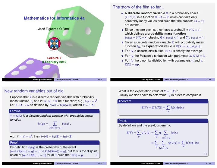
The story of the film so far... A discrete random variable X in a probability space ( Ω , F , P ) is a function X : Ω → R which can take only Mathematics for Informatics 4a countably many values and such that the subsets { X = x } are events. Jos´ e Figueroa-O’Farrill Since they are events, they have a probability P ( X = x ) , which defines a probability mass function f X ( x ) = P ( X = x ) obeying 0 � f X ( x ) � 1 and � x f X ( x ) = 1. Given a discrete random variable X with probability mass function f X , its expectation value is E ( X ) = � x xf X ( x ) . For f X a uniform distribution, E ( X ) is simply the average. For f X the Poisson distribution with parameter λ , E ( X ) = λ . Lecture 7 For f X the binomial distribution with parameters n and p , 8 February 2012 E ( X ) = np . Jos´ e Figueroa-O’Farrill mi4a (Probability) Lecture 7 1 / 25 Jos´ e Figueroa-O’Farrill mi4a (Probability) Lecture 7 2 / 25 New random variables out of old What is the expectation value of Y = h ( X ) ? Luckily we don’t have to determine f Y in order to compute it. Suppose that X is a discrete random variable with probability mass function f x and let h : R → R be a function; e.g., h ( x ) = x 2 . Theorem Let Y : Ω → Z be defined by Y ( ω ) = h ( X ( ω )) , written Y = h ( X ) . � E ( Y ) = E ( h ( X )) = h ( x ) f X ( x ) Lemma x Y = h ( X ) is a discrete random variable with probability mass function Proof. � f X ( x ) . f Y ( y ) = By definition and the previous lemma, { x | h ( x )= y } � � � E ( Y ) = yf Y ( y ) = f X ( x ) y e.g., if h ( x ) = x 2 , then f Y ( 4 ) = f X ( 2 ) + f X (− 2 ) . x y y h ( x )= y � � � Proof. = yf X ( x ) = h ( x ) f X ( x ) x By definition f Y ( y ) is the probability of the event y x h ( x )= y { ω ∈ Ω | Y ( ω ) = y } = { ω ∈ Ω | h ( X ( ω )) = y } , but this is the disjoint union of { ω ∈ Ω | X ( ω ) = x } for all x such that h ( x ) = y . Jos´ e Figueroa-O’Farrill mi4a (Probability) Lecture 7 3 / 25 Jos´ e Figueroa-O’Farrill mi4a (Probability) Lecture 7 4 / 25

Moment generating function Examples A special example of this construction is when h ( x ) = e tx , Let a be a constant. where t ∈ R is a real number. Let Y = X + a . Then 1 Definition � � � E ( Y ) = ( x + a ) f X ( x ) = xf X ( x ) + af X ( x ) = E ( X ) + a The moment generating function M X ( t ) is the expectation x x x value � M X ( t ) := E ( e tX ) = e tx f X ( x ) Let Y = aX . Then 2 x � � (provided the sum converges) E ( Y ) = axf X ( x ) = a xf X ( x ) = a E ( X ) x x Lemma M X ( 0 ) = 1 1 Let Y = a . Then 3 X ( 0 ) , where ′ denotes derivative with respect to t . E ( X ) = M ′ 2 � E ( Y ) = af X ( x ) = a x Jos´ e Figueroa-O’Farrill mi4a (Probability) Lecture 7 5 / 25 Jos´ e Figueroa-O’Farrill mi4a (Probability) Lecture 7 6 / 25 Example Example Let X be a discrete random variable whose probability mass Let X be a discrete random variable whose probability mass function is given by a binomial distribution with parameters n function is a Poisson distribution with parameter λ . Then and p . Then ∞ e − λ λ x � x ! e tx M X ( t ) = n � � n � p x ( 1 − p ) n − x e tx M X ( t ) = x = 0 x x = 0 ∞ e − λ ( λe t ) x � = n � n � � x ! ( e t p ) x ( 1 − p ) n − x = x = 0 x = e λ ( e t − 1 ) . x = 0 = ( e t p + 1 − p ) n . Differentiating with respect to t , Differentiating with respect to t , X ( t ) = e λ ( e t − 1 ) λe t , M ′ X ( t ) = n ( e t p + 1 − p ) n − 1 pe t M ′ whence setting t = 0, M ′ X ( 0 ) = λ , as we had obtained before. whence setting t = 0, M ′ X ( 0 ) = np , as we obtained before. (But again this way is simpler.) (This way seems simpler, though.) Jos´ e Figueroa-O’Farrill mi4a (Probability) Lecture 7 7 / 25 Jos´ e Figueroa-O’Farrill mi4a (Probability) Lecture 7 8 / 25

Variance and standard deviation I Variance and standard deviation II The expectation value E ( X ) (also called the mean ) of a discrete Let X be a discrete random variable with mean µ . The variance random variable is a rather coarse measure of how X is is a weighted average of the (squared) distance from the mean. distributed. For example, consider the following three More precisely, situations: Definition I give you £ 1000 1 The variance Var ( X ) of X is defined by I toss a fair coin and if it is head I give you £ 2000 2 � Var ( X ) = E (( X − µ ) 2 ) = ( x − µ ) 2 f X ( x ) I choose a number from 1 to 1000 and if can guess it, I give 3 x you £ 1 million Let X be the discrete random variable corresponding to your (provided the sum converges.) Its (positive) square root is called the standard deviation and winnings. In all three cases, E ( X ) = £ 1000, but you will agree is usually denoted σ , whence that your chances of actually getting any money are quite different in all three cases. � � ( x − µ ) 2 f X ( x ) One way in which these three cases differ is by the “spread” of σ ( X ) = the probability mass function. This is measured by the variance . x One virtue of σ ( X ) is that it has the same units as X . Jos´ e Figueroa-O’Farrill mi4a (Probability) Lecture 7 9 / 25 Jos´ e Figueroa-O’Farrill mi4a (Probability) Lecture 7 10 / 25 Variance and standard deviation III Another expression for the variance Let us calculate the variances and standard deviations of the Theorem above three situations: If X is a discrete random variable with mean µ , then I give you £ 1000. There is only one outcome and it is the 1 mean, hence the variance is 0. Var ( X ) = E ( X 2 ) − µ 2 I toss a fair coin and if it is head I give you £ 2000. 2 2 ( 2000 − 1000 ) 2 + 1 2 ( 0 − 1000 ) 2 = 10 6 Var ( X ) = 1 Proof. whence σ ( X ) = £ 1, 000. � � I choose a number from 1 to 1000 and if can guess it in ( x 2 − 2 µx + µ 2 ) f X ( x ) 3 ( x − µ ) 2 f X ( x ) = Var ( X ) = one attempt, I give you £ 1 million. x x � � xf X ( x ) + µ 2 � x 2 f X ( x ) − 2 µ = f X ( x ) Var ( X ) = 10 − 3 ( 10 6 − 10 3 ) 2 + 999 × 10 − 3 ( 0 − 10 3 ) 2 ≃ 10 9 x x x = E ( X 2 ) − 2 µ E ( X ) + µ 2 = E ( X 2 ) − µ 2 whence σ ( X ) ≃ £ 31, 607. Jos´ e Figueroa-O’Farrill mi4a (Probability) Lecture 7 11 / 25 Jos´ e Figueroa-O’Farrill mi4a (Probability) Lecture 7 12 / 25

Properties of the variance Variance from the moment generating function Let X be a discrete random variable with moment generating Theorem function M X ( t ) . Let X be a discrete random variable and α a constant. Then Theorem Var ( αX ) = α 2 Var ( X ) and Var ( X + α ) = Var ( X ) X ( 0 ) 2 Var ( X ) = M ′′ X ( 0 ) − M ′ Proof. Proof. Since E ( αX ) = α E ( X ) and E ( X + α ) = E ( X ) + α , Notice that the second derivative with respect to t of M X ( t ) is Var ( αX ) = E ( α 2 X 2 ) − α 2 µ 2 = α 2 Var ( X ) given by d 2 � � x 2 e tx f X ( x ) , e tx f X ( x ) = dt 2 and x x X ( 0 ) = E ( X 2 ) . The result follows from the expression Var ( X + α ) = E (( X + α − ( µ + α )) 2 ) = E (( X − µ ) 2 ) = Var ( X ) whence M ′′ Var ( X ) = E ( X 2 ) − µ 2 and the fact that µ = M ′ X ( 0 ) . Jos´ e Figueroa-O’Farrill mi4a (Probability) Lecture 7 13 / 25 Jos´ e Figueroa-O’Farrill mi4a (Probability) Lecture 7 14 / 25 Example Example Let X be a discrete random variable whose probability mass Let X be a discrete random variable with probability mass function is a binomial distribution with parameters n and p . It function given by a Poisson distribution with mean λ . Its has mean µ = np and moment generating function moment generating function is M X ( t ) = e λ ( e t − 1 ) M X ( t ) = ( e t p + 1 − p ) n Differentiating twice Differentiating twice X ( t ) = n ( n − 1 )( e t p + 1 − p ) n − 2 p 2 e 2 t + np ( e t p + 1 − p ) n − 1 e t , X ( t ) = e λ ( e t − 1 ) λe t + e λ ( e t − 1 ) ( λe t ) 2 M ′′ M ′′ X ( 0 ) = λ + λ 2 and thus X ( 0 ) = n ( n − 1 ) p 2 + np and thus Evaluating at 0, M ′′ Evaluating at 0, M ′′ Var ( X ) = n ( n − 1 ) p 2 + np − ( np ) 2 = np ( 1 − p ) Var ( X ) = λ + λ 2 − λ 2 = λ Jos´ e Figueroa-O’Farrill mi4a (Probability) Lecture 7 15 / 25 Jos´ e Figueroa-O’Farrill mi4a (Probability) Lecture 7 16 / 25