ArDec: Autoregressive-based time series decomposition in R Susana - PowerPoint PPT Presentation
Introduction Method Application Summary ArDec: Autoregressive-based time series decomposition in R Susana Barbosa Universidade do Porto, Portugal : Introduction Method Application Summary Time series decomposition Approaches:
Introduction Method Application Summary ArDec: Autoregressive-based time series decomposition in R Susana Barbosa Universidade do Porto, Portugal :
Introduction Method Application Summary Time series decomposition Approaches: ◮ non-parametric : filtering / smoothing (eg STL, discrete wavelet transform, ...) ◮ model-based : regression, structural models, ... Goals: ◮ remove “known” (non-stationary) components ◮ describe components of interest (seasonal, trend, ...) :
Introduction Method Application Summary Time series decomposition Approaches: ◮ non-parametric : filtering / smoothing (eg STL, discrete wavelet transform, ...) ◮ model-based : regression, structural models, ... Goals: ◮ remove “known” (non-stationary) components ◮ describe components of interest (seasonal, trend, ...) :
Introduction Method Application Summary Trend & seasonality ◮ “The essential idea of trend is that it is smooth. ” ◮ “A trend is a consistent pattern over time. ◮ “A trend is a long-term movement in time series data after other components have been accounted for. “ ◮ “A trend is a trend, is a trend, is a trend, ...” :
Introduction Method Application Summary Trend & seasonality ◮ “the characteristics of a time series giving rise to spectral peaks at seasonal frequencies” [Nerlove 1964] ◮ “the intra-year pattern of variation which is repeated constantly or in an evolving fashion from year to year” [Shiskin et al. 1967] ◮ “periodic fluctuations that recur with about the same intensity each year” [Hillmer and Tiao 1982]. :
Introduction Method Application Summary Problem How to retrieve physically-relevant components? :
Introduction Method Application Summary Problem How to retrieve physically-relevant components? :
Introduction Method Application Summary Method M. West 1997 (Time series decomposition. Biometrika 84) Basic concept: p p γ j � � X t = φ j X t − j + ε t = ⇒ X t = t j = 1 j = 1 :
Introduction Method Application Summary State-space representation of AR(p) process X t = F T Z t Z t = GZ t − 1 + ε t with F T = [ 1 0 ... 0 ] Z T t = [ X t X t − 1 ... X t − p + 1 ] φ 1 φ 2 ... φ p 1 0 ... 0 G = . . ... . . . 1 . 0 :
Introduction Method Application Summary State-space representation of AR(p) process X t = F T Z t Z t = GZ t − 1 + ε t G = EAE − 1 − → r j e ± iw j a = E T F , b t = E − 1 Z t X t = � p j = 1 γ j t , γ j t = a j b j t → γ j w j = 0 − t = r j γ t − j + ν t → γ j t = 2 r j cos ( w j ) γ j t − 1 + r 2 j γ j w j � = 0 − t − 2 + η t :
Introduction Method Application Summary Decomposition of sea-level records with ArDec :
Introduction Method Application Summary Decomposition of sea-level records with ArDec ❃ ❧✐❜r❛r②✭❆r❉❡❝✮ ❃ ❝♦❡❢❂❛r❞❡❝✳❧♠✭❞❛t✮✩❝♦❡❢❢✐❝✐❡♥ts ❃ ❝♦❡❢ ❳✶ ❳✷ ❳✸ ❳✹ ❳✺ ❳✻ ✵✳✸✽✻✶✽✻✹✹✻ ✵✳✵✺✵✵✵✼✺✸✻ ✵✳✵✽✽✻✹✸✹✺✾ ✵✳✵✵✷✼✸✵✵✵✹ ✵✳✵✹✺✾✶✺✷✺✵ ✲✵✳✵✵✾✺✸✾✻✹✺ ❳✼ ❳✽ ❳✾ ❳✶✵ ❳✶✶ ❳✶✷ ✵✳✵✺✽✶✸✼✺✽✽ ✵✳✵✸✷✵✶✺✽✾✼ ✲✵✳✵✼✺✸✼✽✼✵✾ ✵✳✵✻✹✽✹✼✹✹✵ ✵✳✶✶✼✼✵✺✾✺✾ ✵✳✶✻✾✸✷✷✼✽✸ ❳✶✸ ❳✶✹ ❳✶✺ ❳✶✻ ❳✶✼ ❳✶✽ ✵✳✵✻✵✷✽✽✽✽✾ ✲✵✳✵✼✼✻✷✶✻✹✵ ✲✵✳✵✼✹✽✽✵✺✾✵ ✲✵✳✵✶✷✾✶✶✷✷✸ ✵✳✵✶✵✽✻✾✵✹✸ ✲✵✳✵✵✾✼✹✷✼✸✷ ❳✶✾ ❳✷✵ ❳✷✶ ❳✷✷ ❳✷✸ ❳✷✹ ✲✵✳✵✹✽✹✾✾✻✸✻ ✲✵✳✵✵✷✻✹✸✺✵✺ ✲✵✳✵✹✹✹✷✷✼✷✷ ✵✳✵✺✹✻✾✽✸✼✷ ✵✳✵✺✷✺✷✾✶✹✼ ✵✳✶✸✾✽✹✾✼✻✾ ❳✷✺ ❳✷✻ ✵✳✵✼✷✽✵✸✽✸✻ ✲✵✳✵✽✶✻✽✼✶✵✹ :
Introduction Method Application Summary Decomposition of sea-level records with ArDec ❃ ❛r❞❡❝✭❞❛t✱❝♦❡❢✮ ♣❡r✐♦❞ ❞❛♠♣✐♥❣ ✶ ✧tr❡♥❞✧ ✧✵✳✾✾✻✧ ✷ ✧✶✷✳✵✽✾✧ ✧✵✳✾✽✻✧ ✸ ✧✻✳✵✵✵✧ ✧✵✳✾✽✷✧ :
Introduction Method Application Summary Decomposition of sea-level records with ArDec ❃ str✭❛r❞❡❝✳❝♦♠♣♦♥❡♥ts✭❛r❞❡❝✳♦✉t✮✮ ▲✐st ♦❢ ✷ ✩ ♣❡r✐♦❞❝♦♠♣s✿▲✐st ♦❢ ✷ ✳✳✩ ♣❡r✐♦❞s✿ ♥✉♠ ❬✶✿✷❪ ✶✷✳✶ ✻✳✵ ✳✳✩ ❝♦♠♣s ✿ ♠ts ❬✶✿✾✸✻✱ ✶✿✷❪ ◆❆ ◆❆ ◆❆ ◆❆ ◆❆ ◆❆ ◆❆ ◆❆ ◆❆ ✳✳✳ ✳✳ ✳✳✲ ❛ttr✭✯✱ ✧❞✐♠♥❛♠❡s✧✮❂▲✐st ♦❢ ✷ ✳✳ ✳✳ ✳✳✩ ✿ ◆❯▲▲ ✳✳ ✳✳ ✳✳✩ ✿ ❝❤r ❬✶✿✷❪ ✧❙❡r✐❡s ✶✧ ✧❙❡r✐❡s ✷✧ ✳✳ ✳✳✲ ❛ttr✭✯✱ ✧ts♣✧✮❂ ♥✉♠ ❬✶✿✸❪ ✶✾✷✽ ✷✵✵✻ ✶✷ ✳✳ ✳✳✲ ❛ttr✭✯✱ ✧❝❧❛ss✧✮❂ ❝❤r ❬✶✿✷❪ ✧♠ts✧ ✧ts✧ ✩ tr❡♥❞❝♦♠♣ ✿ ❚✐♠❡✲❙❡r✐❡s ❬✶✿✾✸✻❪ ❢r♦♠ ✶✾✷✽ t♦ ✷✵✵✻✿ ◆❆ ◆❆ ✳✳✳ :
Introduction Method Application Summary Decomposition of sea-level records with ArDec :
Introduction Method Application Summary Chesapeake bay :
Introduction Method Application Summary Chesapeake bay: annual components :
Introduction Method Application Summary Chesapeake bay: trend components :
Introduction Method Application Summary Package ArDec ◮ implements autoregressive-based time series decomposition ◮ model-based, additive decomposition ◮ yields periods of physically-relevant (non-damped) components ◮ extracts flexible, time-varying estimates of such components ◮ option of Bayesian framework for autoregressive estimation :
Introduction Method Application Summary Thanks! :
Recommend
More recommend
Explore More Topics
Stay informed with curated content and fresh updates.
![Autoregressive Models Autoregressive Models In [1]: from mxnet import autograd, nd, gluon, init](https://c.sambuz.com/996111/autoregressive-models-autoregressive-models-s.webp)

