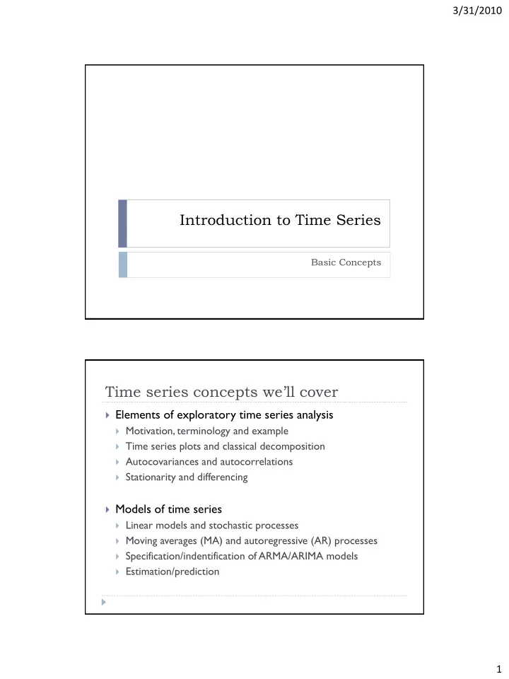
Introduction to Time Series Basic Concepts Time series concepts - - PDF document

3/31/2010 1

Introduction to Time Series

Basic Concepts

Time series concepts we’ll cover

 Elements of exploratory time series analysis

 Motivation, terminology and example  Time series plots and classical decomposition  Autocovariances and autocorrelations  Stationarity and differencing

 Models of time series

 Linear models and stochastic processes  Moving averages (MA) and autoregressive (AR) processes  Specification/indentification of ARMA/ARIMA models  Estimation/prediction

3/31/2010 2

Lecture objectives

 Understand the goals of TS analysis  Talk about TS terminology  Examine a simple example of a TS analysis  Conduct simple exploratory TS analysis using plots and

decomposition techniques

 Discuss the concepts of autocovariance and

autocorrelation and how they can be used to examine TS processes

Definition

 A time series is a record of values of a certain variable of

interest taken at different points in time

 Data are observed at equally spaced time intervals

 Discrete-time time series

 Method of measurement should be consistent over time  Notation: Xt is the measurement of variable X at time t

 Xt can be continuous or discrete (counts)

3/31/2010 3

Time Series Analysis

 A time series can be decomposed into its components:

trend, cycles (including seasonal) and irregular components:

 This idea is very old and is now out of favor but it is still

widely used

n explanatio no have we for which effect random S period a with component seasonal

• r

cyclical series the

• f

componded trend t at time series the

• f

value : where       

t t t t t t t t

R S T X R S T X

t t t t t

R C S T X     : OR

3/31/2010 4

Overview of time series analysis

 Goal in analyzing a particular time series is to:

 Make a forecast  Understand the underlying mechanism

 Start with building a model for the data

 Method for “reducing” the series to some kind of standard

“random noise”

 For forecasting, the utility of the “reduction to random

noise” notion is that “noise” cannot be predicted

 We can then reverse the “reduction to random noise”

procedure to obtain a prediction for the original series

 In regression analysis, what is the noise?

Overview of time series analysis

 Since “noise” is not understandable, all the useful

information is in the trend, seasonality, etc.

 Construct a series from simple assumptions about each of the

individual components

 Three typical steps in the “reduction-to-noise'' process:

 A data transformation such as taking logarithms of the data  Removing seasonality and trend to obtain a stationary process.  Fit a standard time series model

 The “reduction-to-noise” procedure does not always

proceed in a linear fashion

 One will usually jump around from one attempt after another

• f trying to develop each of the three components

3/31/2010 5

Applications

 Geosciences and meteorology

 weather forecasting, trends in weather patterns

 Business and finance (econometrics)

 stock market analysis, business forecasting

 Multivariate statistical data analysis

 RS image analysis

 Medicine

 epidemic analysis

Goals depend on the study question

 Climatologist interested in global warming

 Interested in the long term trend of CO2 or temperature, so

ignores the seasonal/daily/monthly cycles

 Economist interested in demand for electricity

 Interested in the long term trends (due to population growth?

global warming?) but also the daily/monthly/seasonal peaks

 Epidemiologist interested in preparing for the flu season

 Not really interested in long term trends at all, interested in

monthly/seasonal cycle and error (abnormal spikes in flu rates)

3/31/2010 6

Steps in a classical time series analysis

1.

Do a time plot of the time series

2.

Describe the variability of the series seen in the plot:

 Is there a trend? Is the trend in mean and variance? Or only one of

them?

 Is there a seasonal pattern? What is the period?  Is there any additional irregular variability?

3.

Use time series plots to determine whether transformations are necessary

4.

Transform the data if necessary



Log or square root transforms

Steps in a classical time series analysis

5.

Use time plots and test statistics to determine if the series is stationary (constant mean and or variance)

6.

Make the series stationary if it is not

7.

Fit TS model to series and analyze residuals

8.

When a good model is found, forecast the future

3/31/2010 7

Terminology

 Dependence: Correlation of observations of one variable

at one point in time with observations of the same variable at prior points in time

 Serial correlation or autocorrelation

 Stationarity: The mean value of the series remains

constant over the time series (e.g., no systematic change in the mean, no trend)

 Also, variance should remain constant

Terminology

 Differencing: data pre-processing step which de-trends

the data to achieve stationarity

 Subtract each data point in a series from it’s predecessor  Most methods in TS analysis are concerned with stationary

time series

 Specification: using diagnostic tests, specifying the type of

time series model to apply to the series

 Auto-regressive (AR), Moving average (MA), ARMA (combined)

• r ARIMA (combined integrated)

 Also could have non-linear models

3/31/2010 8

What is a trend?

 A trend is a long term change in the mean and/or

variance of the series

 e.g., if you computed the mean of the series at several different

intervals, the mean would be different in each

 Trends can be increasing or decreasing, and can have

many function forms

 Global linear trends (generally unrealistic)  Piecewise linear (local linear)  Nonlinear

 Exponential  Quadratic or other polynomial

...

2 

  

   s t s t t s t

X X X X

Identifying a trend

 If the trend is not immediately apparent (usually due to a

large error component) we can identify it using a smoothing process:

 No huge outliers – moving averages  Considerable error – exponential smoothing

 Once we have identified the trend we can model it:

 Fit a linear regression model to the data  Fit another type of function to the data

 Polynomial curve (quadratic, etc)  Logistic curve

3/31/2010 9

Analyzing the trend

 Most time series methods require stationary data

 We need to transform nonstationary series before modeling

 We can remove a trend through a process called

differencing

 Fit a linear/quadratic/polynomial function to the trend and

subtract the fitted values from each observation

 RESIDUALS

 Subtract each observation from it’s neighbor (Xt-Xt-1)

 Often the whole point of modeling a trend is to create a

residual series that is used for time series analysis

Example of a trend model

 The simplest trend model for a linear trend

 If  and  are assumed constants, the trend is called

deterministic

 If  and  are assumed random, then the trend is stochastic

t at time series the

• f

mean n) 1,2,..., (t index time t mean with error term random t at time series the

• f

value

• bserved

: where          t X t X

t t t t

     

3/31/2010 10

Example

 Consider the time series above

 It has an upward trend and some seasonal effect.  It doesn’t show increasing variation in amplitude over time  Let’s concentrate on the trend

 It could be linear, so we fit a line using regression

Example

t T 017 . 92 . 34 ˆ   

3/31/2010 11

Detrending the data

 Once we have found a trend model, we can use the

model to predict future values, or to detrend the data

 To detrend the data:

 Detrended data = Xt - fitted trend (residuals)

Detrending the data

 Detrended data  The detrended data has still the seasonal (S) and the

irregular (ε) components

 However, this type of line often does not capture the

trend well because the trend is not quite linear

 To fix this distortion, a different type of detrending model (e.g.,

moving average) can be used to capturing the trend

) 017 . 92 . 34 ( ˆ t X T X

t t

     

3/31/2010 12

Seasonality

 Variation (increase or decrease in the series) that is

annual in period

 Rainfall, temperature, ice melt, swimsuit sales

 The seasonality can be measured or estimated, if it is of

direct interest

 Alternatively, seasonality can be removed to give

seasonally adjusted data (differencing)

 The logic is that we already know that effect is there, so

remove it to see what other things are relevant in the data

Types of seasonality

 Seasonality can be additive, which means that it is

constant from year to year

 e.g., each year rainfall increases approximately the same

amount due to the summer/winter effect

error random t at time effect seasonal t at time series the

• f

level mean the t at time series the

• f

value the : where       

t t t t t t t t

S T X S T X  

3/31/2010 13

Types of seasonality

 Seasonality can be multiplicative, which means that the

seasonality is proportional to the mean of the series

 There are two types of multiplicative seasonality

 (a) Multiplicative seasonality with additive error term  (b) Multiplicative seasonality with multiplicative error

 A logarithmic transformation will convert the series to

additive seasonality

t t t t

S T X    *

t t t t

S T X  * * 

Estimating the seasonality

 We first need to identify the seasonal components (what

is the period and/or cycle)

 Smooth the series

 Once we have identified the seasonal component we can

model it:

 Simple differencing (Xt-Xt-12)  Moving average (12-month)  Linear model (with a factor/variable for season)  Harmonic function (series of sin/cos functions)

3/31/2010 14

Example

 There may be a

seasonal effect (roughly) corresponding to a yearly cycle

Example

 The period is s=12  After applying a 12-point moving average, we obtained the

smooth series overimposed

3/31/2010 15

Removing seasonality

 In most cases, we estimate the seasonality not to use it to

put in the model used for forecasting, but simply to remove it

 To remove it, we choose some type of model that

estimates the seasonal effect

 Linear model with factors for season

 Both trend and seasonality  Xt=Time+Season  Then we look at the residuals

 Residuals = error

Fitted model

 Once we have the seasonal element estimated, we can

add them to the trend fitted earlier to obtain the predicted values or fitted model

t t t

S T X  

3/31/2010 16

Random error

 Once we detrend and remove seasonality, all that is left is

the random or error component

 Appears stationary, so we can use this in TS models

To make a series X stationary

1.

Check if there is variance that changes with time

 Make variance constant with log or square root transformation  Call the transformed data X*

2.

Remove the trend in mean with regular differencing or fitting a trend line

 Call the new series X**  The correlogram of X** should only have a few significant spikes at

small lags 3.

If there is a seasonal cycle left in the data, we must seasonally difference the series too

 Call the new series X**

3/31/2010 17

What have we learned so far?

 We used a rather rough way of estimating trend and

seasonality, which are components of the additive decomposition model

 We have used those components to fit a model and to

detrend and seasonally adjust the series

 No attempt was made to see the accuracy of any of the

things estimated

 No statistics, really

 In doing all this, we introduced the notions of trend,

seasonality, irregular components, fitted model

 These concepts will reappear over and over with the different

methods used

Descriptive Analysis

3/31/2010 18

Steps in classical time series analysis

1.

Do a time plot of the time series

2.

Describe the variability of the series seen in the plot:

 Is there a trend? Is the trend in mean and variance? Or only one of

them?

 Is there a seasonal pattern? What is the period?  Is there any additional irregular variability?

3.

Use time series plots to determine whether transformations are necessary

4.

Transform the data if necessary



log or square root transforms, or generalized Box-Cox transforms

Plotting

 Import our data file  Transform it into a time series object in R

> mloa<-read.table("C:/Users/Eroot/Quant/R/monaloa.txt", header=T, sep=",") > names(mloa) [1] "year" "month" "mean" "interp" > mlco2<-ts(mloa$interp, st=c(1958,3), end=c(2010,1), fr=12) > plot(mlco2, ylab="Mean CO2 (PPM)") > ts.plot(mloa$interp, ylab="Mean CO2 (PPM)")

3/31/2010 19

Example: Mona Loa CO2 concentrations Plotting

 One way to look at seasonality

> boxplot(mlco2~cycle(mlco2))

3/31/2010 20

Classical decomposition

> mlco2.dec<-decompose(mlco2, type="mult") > plot(mlco2.dec)

Plotting

 What does non-stationary variance look like?

3/31/2010 21

Transforming

> logAP<-log(AP) > plot(logAP, ylab="Air Passengers (1000s)")

Time series and autocorrelation

 Time series are different from other data studied most

stats courses because the observations tend to be correlated

 Just like the spatial data we’ve been discussing for the past

month!

 We say that the data has memory: observations today are

affected by what happened in the past

 The question is: How correlated are the observations

with each other? How far does the memory go?

3/31/2010 22

Time series and autocorrelation

 Compute the correlation coefficient between the value of

the time series at time t and its value at time t-1

 Analogous to the simple correlation coefficient (r)  But instead of correlation between 2 different variables,

compute correlation between same variable at 2 points in time (xt, xt+1)

 So, the autocorrelation coefficient at lag 1 calculated using

N-1 pairs of data

 (x1, x2), (x2, x3), (x3, x4), etc.

 

   

    

N t t N t t t

N x x N x x x x r

1 2 1 1 1 1

/ ) ( ) 1 ( ) )( (

Time series and autocorrelation

 But the memory of the data might go past the

• bservation at time t-1!

 How is the observation at time t correlated with that at time t-

2? Or at time t-3? Or at time t-k?

 Need to compute the autocorrelation coefficient at lag 2

(r2) using N-2 pairs

 (x1, x3), (x2, x4), …, (xN-2, xN)

 And at lag 3 (r3) using N-3 pairs

 (x1, x4), (x2, x5), …, (xN-3, xN)

3/31/2010 23

Example Plotting autocorrelation

 We can look at scatter plots of xt vs. xt+1 Correlation at lag 1 r1 = 0.60; p<0.001 Correlation at lag 2 r1 = 0.09; p=0.06

3/31/2010 24

The correlogram

 We could compute autocorrelations at other lags by

hand…but this is tedious!

 The correlogram is a summary statistic for a time series that

tells us the autocorrelation coefficients rk at lags k

 Visual inspection of the correlogram gives us hints about the

nature of our time series

 Random series  Short-term correlation  Non-stationary series  Seasonal series

 Helps us identify which type of ARIMA model to use

Example

95% CI around the null hypothesis for rn=0 r2=0.6 r3=0.1

3/31/2010 25

Interpretation of the correlogram Interpretation of the correlogram…

3/31/2010 26

Interpretation of the correlogram Interpretation of the correlogram