Introduction to Time Series Heino Bohn Nielsen 1 of 15 Outline - - PDF document

SLIDE 1

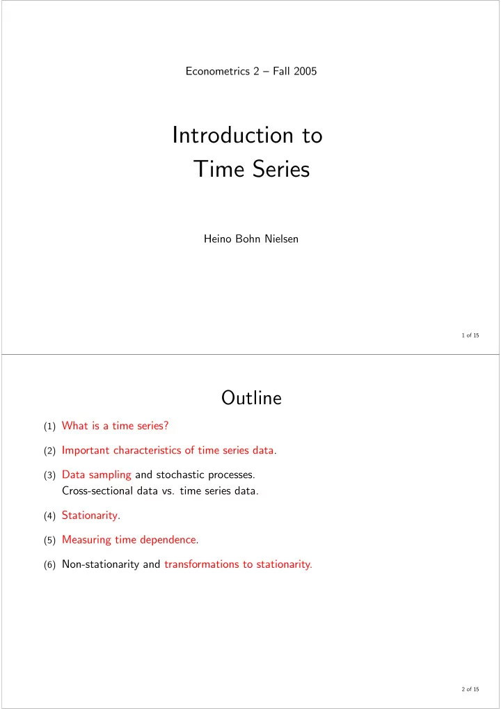
Econometrics 2 — Fall 2005

Introduction to Time Series

Heino Bohn Nielsen

1 of 15

Outline

(1) What is a time series? (2) Important characteristics of time series data. (3) Data sampling and stochastic processes.

Cross-sectional data vs. time series data.

(4) Stationarity. (5) Measuring time dependence. (6) Non-stationarity and transformations to stationarity.

2 of 15

SLIDE 2

Time Series Data

• A time series is a set of observations

y1, y2, ..., yt, ..., yT,

where t is the time index. Natural temporal ordering.

• It holds that yt−1 is observed when yt is determined.

Focus on conditional models yt | yt−1, yt−2, ....

• Most data in macro-economics and finance come in this form.
• Very different characteristics.

The tools should match the characteristics of the data.

3 of 15

Characteristics of Time Series Data

1970 1980 1990 2000 0.25 0.50 0.75 1.00 (B) Danish productivity (logs) 1950 1960 1970 1980 1990 2000 0.0 2.5 5.0 7.5 10.0 12.5 (A) US unemployment rate 150 300 450 600 750 900 1050

• 10
• 5

5 10 (D) Daily change in the NASDAQ index (%)

Period: 3/1-2000 to 26/2-2004

1970 1980 1990 2000 5.9 6.0 6.1 6.2 6.3 6.4 (C) Danish income and consumption (logs) Income Consumption

4 of 15

SLIDE 3

Random Sampling (Cross-Sectional Data)

• The observations x1, ..., xN are randomly drawn from a fixed population.

N Observations from the same distribution. No ordering.

• When N is large we can characterize the distribution.

Law of large numbers: N−1 XN

i=1 xi → E[xi].

y y1 y3 y2 y8 y7y4 y9 y6 y5 Random sampling from population Sample distribution approximates the population y

5 of 15

Stochastic Processes (Time Series Data)

• Observation yt is a realization of a random variable yt.

Only one observation per random variable!

• The sequence of random variables y1, ..., yT is denoted a stochastic process.

t 1 2 3 4 5 6 7 y

6 of 15

SLIDE 4

• If we could rerun history M times:

Stochastic process:

y1, y2, ..., yt, ..., yT

Realization 1 :

y(1)

1 ,

y(1)

2 ,

..., y(1)

t ,

..., y(1)

T

. . . . . . . . . . . . Realization m :

y(m)

1

, y(m)

2

, ..., y(m)

t

, ..., y(m)

T

. . . . . . . . . . . . Realization M :

y(M)

1

, y(M)

2

, ..., y(M)

t

, ..., y(M)

T

.

• Consider the ensemble mean, E[yt], estimated with the average

b E[yt] = 1 M

M

X

m=1

y(m)

t

.

• Fundamentally different from the time average of a realized sample path

y = 1 T

T

X

t=1

y(1)

t .

7 of 15

Stationarity

• A time series, y1, y2, ..., yt, ..., yT, is called strictly stationary if the distributions

(yt1, yt2, ..., ytn)

and

(yt1+h, yt2+h, ..., ytn+h)

are the same for all h. The distribution of yt does not depend on t.

• The time series is called weakly stationary if

E[yt] = µ V [yt] = E[(yt − µ)2] = γ0 Cov[yt, yt−k] = E[(yt − µ) (yt−k − µ)] = γk

for k = 1, 2, ...

t 1 2 3 4 5 6 7 y

8 of 15

SLIDE 5

Main Result

Stationarity implies that yt (t = 1, 2, ..., T) contain information on the same distribution. And yt fluctuates around a constant level: equilibrium correcting.

• We make the additional assumption that yt and yt−k becomes approximately inde-

pendent for k → ∞. This technical assumption called weak dependence, ensures that a law of a large numbers (LLN) hold. Then y is a consistent estimator of E[yt].

• Given stationarity and weak dependence of yt and xt, most properties of OLS in the

IID case carry over to the time series regression

yt = x0

tβ + t.

We return to this issue later. The most important distinction in time series econometrics is whether the time series of interest are stationary or not.

9 of 15

Measuring Time Dependence

A characteristic feature of time series is a clear dependence over time. We can measure the dependence by the correlation Corr(yt, yt−k) =

Cov(yt, yt−k) p V (yt) · V (yt−k) , k = ..., −2, −1, 0, 1, 2, ...

Under stationarity the formula simplifies to the so-called autocorrelation function (ACF)

ρk = Cov(yt, yt−k) V (yt) , k = ..., −2, −1, 0, 1, 2, ...

which can be estimated by e.g.

b ρk =

1 T−k

XT

t=k+1 (yt − y) (yt−k − y) 1 T−k

XT

t=k+1 (yt−k − y)2

.

10 of 15

SLIDE 6

Empirical Example

Look at the US unemployment rate.

• It is not clear whether ut equilibrium corrects.
• It fluctuates within bounds, but deviations are very persistent and equilibrium cor-

rection is very slow. ut and ut−k are highly correlated for large values if k.

• We return to formal testing later.

1950 1960 1970 1980 1990 2000 5.0 7.5 10.0 (A) US unemployment rate 5 10 15 0.5 1.0 (B) ACF for (A)

11 of 15

Transformation to Stationarity

Many economic time series are not stationary. Sometimes, a non-stationary time series can be transformed to stationarity. Three important cases: (A) Remove a deterministic trend. Trend stationary. (B) Take first differences. Difference stationary or integrated or first order. (C) Combine several variables. Cointegration.

12 of 15

SLIDE 7

(A) If the non-stationary of yt is due to a deterministic trend, then the de-trended variable

y∗

t = yt − µ0 − µ1t,

might be stationary. In this case, yt is called trend-stationary. The de-trended variable can be found as the estimated residual in the linear regression

yt = µ0 + µ1t + y∗

t .

As an example look at the Danish productivity.

1970 1980 1990 2000

• 0.05

0.00 0.05 (C) Danish productivity (log) minus trend 5 10 15 0.5 1.0 (D) ACF for (C)

13 of 15

(B) Alternatively it might turn out that yt is non-stationary while the first difference,

∆yt = yt − yt−1,

is stationary. In this case, yt is difference stationary or integrated of first order, I(1). As an example look at Danish private consumption.

1970 1980 1990 2000

• 0.05

0.00 0.05 (E) change in Danish consumption (log) 5 10 15 1 (F) ACF for (E)

14 of 15

SLIDE 8

(C) Finally, it might turn out that two variables, yt and xt, are non-stationary, but related so that a linear combination

zt = yt − β · xt,

is stationary. Here yt and xt are I(1) but so-called co-integrated. As an example consider consumption, ct, and income, yt. Both are I(1) and have no

• equilibrium. They are related, however, and the savings rate,

st = yt − ct,

seems to be stationary and equilibrium corrects.

1970 1980 1990 2000 0.00 0.05 0.10 0.15 (G) Danish savings rate (log) 5 10 15 1 (H) ACF for (G)

15 of 15