Statistical Decision Theory Overview Definitions Experiment: process - PowerPoint PPT Presentation

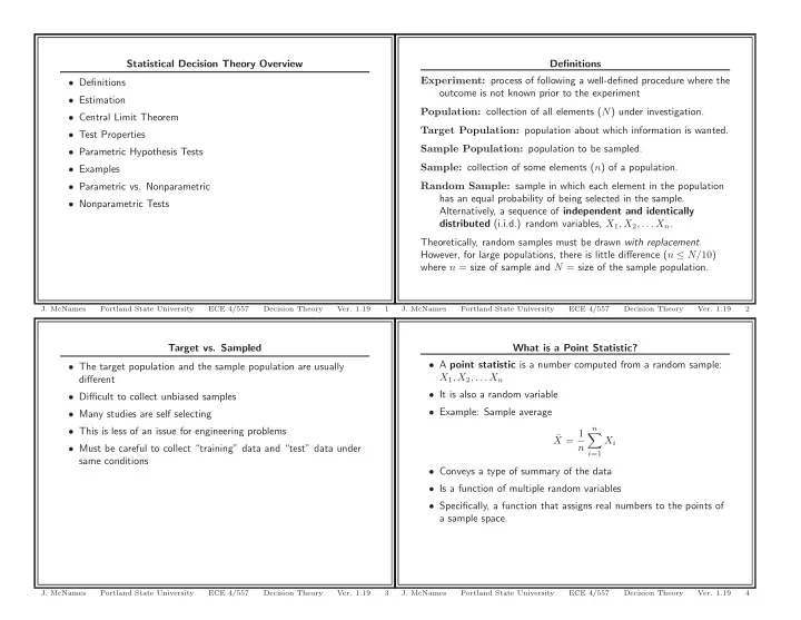
Statistical Decision Theory Overview Definitions Experiment: process of following a well-defined procedure where the • Definitions outcome is not known prior to the experiment • Estimation Population: collection of all elements ( N ) under investigation. • Central Limit Theorem Target Population: population about which information is wanted. • Test Properties Sample Population: population to be sampled. • Parametric Hypothesis Tests Sample: collection of some elements ( n ) of a population. • Examples • Parametric vs. Nonparametric Random Sample: sample in which each element in the population has an equal probability of being selected in the sample. • Nonparametric Tests Alternatively, a sequence of independent and identically distributed (i.i.d.) random variables, X 1 , X 2 , . . . X n . Theoretically, random samples must be drawn with replacement . However, for large populations, there is little difference ( n ≤ N/ 10 ) where n = size of sample and N = size of the sample population. J. McNames Portland State University ECE 4/557 Decision Theory Ver. 1.19 1 J. McNames Portland State University ECE 4/557 Decision Theory Ver. 1.19 2 Target vs. Sampled What is a Point Statistic? • A point statistic is a number computed from a random sample: • The target population and the sample population are usually X 1 , X 2 , . . . X n different • It is also a random variable • Difficult to collect unbiased samples • Example: Sample average • Many studies are self selecting n • This is less of an issue for engineering problems X = 1 ¯ � X i n • Must be careful to collect “training” data and “test” data under i =1 same conditions • Conveys a type of summary of the data • Is a function of multiple random variables • Specifically, a function that assigns real numbers to the points of a sample space. J. McNames Portland State University ECE 4/557 Decision Theory Ver. 1.19 3 J. McNames Portland State University ECE 4/557 Decision Theory Ver. 1.19 4

More Definitions Example 1: MATLAB’s Prctile Function Order Statistic of rank k , X ( k ) : statistic that takes as its value 11 the k th smallest element x ( k ) in each observation ( x 1 , x 2 , . . . x n ) 10 of ( X 1 , X 2 , . . . X n ) 9 p th Sample Quantile: number Q p that satisfies 8 1. The fraction of X i s that are strictly less than Q p is ≤ p 7 pth percentile 2. The fraction of X i s that are strictly greater than Q p is ≤ 1 − p . 6 • If more than one value meets criteria, choose average of 5 smallest and largest. 4 • There are other estimates of quantiles that do not assign 0% 3 and 100% to the smallest and largest observations 2 1 0 0 10 20 30 40 50 60 70 80 90 100 p (%) J. McNames Portland State University ECE 4/557 Decision Theory Ver. 1.19 5 J. McNames Portland State University ECE 4/557 Decision Theory Ver. 1.19 6 Example 1: MATLAB Code Sample Mean and Variance function [] = PrctilePlot(); Sample Mean: n FigureSet(1,’LTX’); µ X = 1 ¯ � X = ˆ X i p = 0:0.1:100; n y = prctile(1:10,p); i =1 h = plot(p,y); set(h,’LineWidth’,1.5); Sample Variance: xlim([0 100]); ylim([0 11]); xlabel(’p (%)’); n ylabel(’pth percentile’); 1 box off; � ( X i − ¯ s 2 σ 2 X ) 2 X = ˆ X = grid on; n − 1 i =1 AxisSet(8); print -depsc PrctilePlot; Sample Standard Deviation: � s 2 s X = ˆ σ X = X J. McNames Portland State University ECE 4/557 Decision Theory Ver. 1.19 7 J. McNames Portland State University ECE 4/557 Decision Theory Ver. 1.19 8

Point vs. Interval Estimators Biased Estimation • Our discussion so far has generated point estimates • An estimator ˆ θ is an unbiased estimator of the population parameter θ if E[ˆ θ ] = θ • Given a random sample, we estimate a single descriptive statistic • Sample mean of a random sample is an unbiased estimate of • Usually preferred to have interval estimates population (true) mean – Example: “We are 95% confident the unknown mean lies X ) 2 is unbiased estimate � n i =1 ( X i − ¯ between 1.3 and 2.7.” • Sample variance s 2 1 X = n − 1 of true (population) variance – Usually more difficult to obtain 1 – Why n − 1 ? – Consist of 2 statistics (each endpoint of the interval) and a – We lose one degree of freedom by estimating E[ X ] with ¯ confidence coefficient X • Also called a confidence interval – Is one of your homework problems • s X is a biased estimate of the true population standard deviation J. McNames Portland State University ECE 4/557 Decision Theory Ver. 1.19 9 J. McNames Portland State University ECE 4/557 Decision Theory Ver. 1.19 10 Central Limit Theorem Central Limit Theorem Continued Let Y n be the sum of n i.i.d. random variables X 1 , X 2 , . . . , X n , let • For large sums, the normal approximation is frequently used µ Y n be the mean of Y n , and σ 2 Y n be the variance of Y n . As n → ∞ , instead of the exact distribution the distribution of the z -score • Also “works” empirically when X i not identically distributed Z = Y n − µ Y n • X i must be independent σ Y n • For most data sets, n = 30 is generally accepted as large enough approaches the standard normal distribution. for the CLT to apply • In many cases, it is assumed that the random sample was drawn • This is remarkable considering the theorem only applies as n → ∞ from a normal distribution • The center of the distribution becomes normally distributed more • This is justified by the central limit theorem (CLT) quickly (i.e., with smaller n ) than the tails • There are many variations • Key conditions: 1 RV’s X i must have finite mean 2 RV’s must have finite variance • RV’s can have any distribution as long as they meet this criteria J. McNames Portland State University ECE 4/557 Decision Theory Ver. 1.19 11 J. McNames Portland State University ECE 4/557 Decision Theory Ver. 1.19 12

Example 2: Central Limit Theorem for Binomial RV Example 3: CLT Applied to Binomial RV σ 2 E[ Y ] = np Y = np (1 − p ) Normalized Binomial Histogram for z N:2 NS:1000 5 Binomial Estimated Gaussian 4.5 • A sum of Bernoulli random variables, Y = � n i =1 X i , has a 4 binomial distribution 3.5 • X i are Bernoulli random variables that take on either a 1 with PDF Estimate 3 probability p or a 0 with probability 1 − p 2.5 • Define Z = Y − E[ Y ] 2 σ Y 1.5 • Let us approximate the PDF of Z from a random sample of 1000 1 points 0.5 • How good is the PDF of Z approximated by a normal distribution? 0 −1.5 −1 −0.5 0 0.5 1 1.5 J. McNames Portland State University ECE 4/557 Decision Theory Ver. 1.19 13 J. McNames Portland State University ECE 4/557 Decision Theory Ver. 1.19 14 Example 3: CLT Applied to Binomial RV Example 3: CLT Applied to Binomial RV Normalized Binomial Histogram for z N:5 NS:1000 Normalized Binomial Histogram for z N:10 NS:1000 3.5 Binomial Estimated Binomial Estimated 2.5 Gaussian Gaussian 3 2 2.5 PDF Estimate PDF Estimate 2 1.5 1.5 1 1 0.5 0.5 0 0 −2.5 −2 −1.5 −1 −0.5 0 0.5 1 1.5 2 2.5 −3 −2 −1 0 1 2 3 J. McNames Portland State University ECE 4/557 Decision Theory Ver. 1.19 15 J. McNames Portland State University ECE 4/557 Decision Theory Ver. 1.19 16

Example 3: CLT Applied to Binomial RV Example 3: CLT Applied to Binomial RV Normalized Binomial Histogram for z N:20 NS:1000 Normalized Binomial Histogram for z N:30 NS:1000 1.6 Binomial Estimated Binomial Estimated 2 Gaussian Gaussian 1.4 1.8 1.6 1.2 1.4 PDF Estimate PDF Estimate 1 1.2 0.8 1 0.8 0.6 0.6 0.4 0.4 0.2 0.2 0 0 −4 −3 −2 −1 0 1 2 3 −3 −2 −1 0 1 2 3 J. McNames Portland State University ECE 4/557 Decision Theory Ver. 1.19 17 J. McNames Portland State University ECE 4/557 Decision Theory Ver. 1.19 18 Example 3: CLT Applied to Binomial RV Example 3: CLT Applied to Binomial RV Normalized Binomial Histogram for z N:100 NS:1000 Normalized Binomial Histogram for z N:1000 NS:1000 0.9 Binomial Estimated Binomial Estimated Gaussian Gaussian 0.5 0.8 0.7 0.4 0.6 PDF Estimate PDF Estimate 0.5 0.3 0.4 0.2 0.3 0.2 0.1 0.1 0 0 −4 −3 −2 −1 0 1 2 3 4 −3 −2 −1 0 1 2 3 4 J. McNames Portland State University ECE 4/557 Decision Theory Ver. 1.19 19 J. McNames Portland State University ECE 4/557 Decision Theory Ver. 1.19 20