Learning unknown forces in nonlinear models with Gaussian processes - PowerPoint PPT Presentation

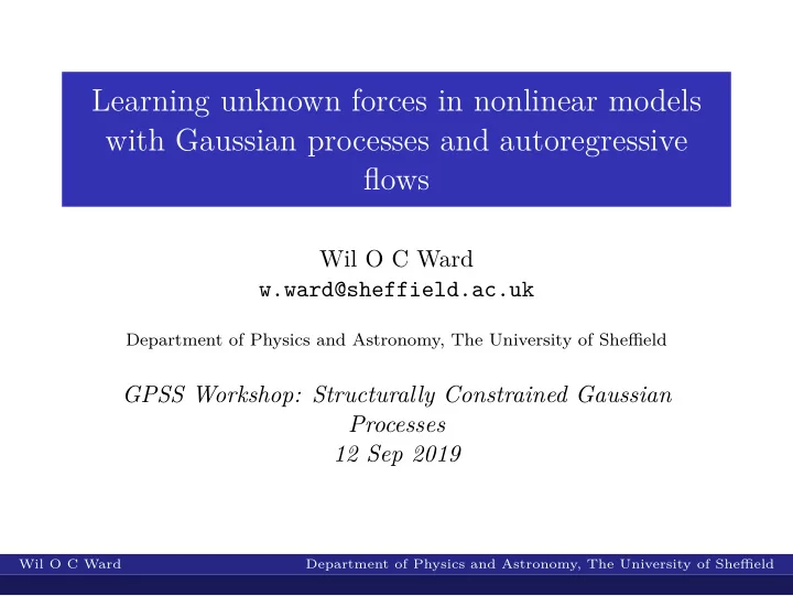
Learning unknown forces in nonlinear models with Gaussian processes and autoregressive flows Wil O C Ward w.ward@sheffield.ac.uk Department of Physics and Astronomy, The University of Sheffield GPSS Workshop: Structurally Constrained Gaussian Processes 12 Sep 2019 Wil O C Ward Department of Physics and Astronomy, The University of Sheffield

Collaborative Work Mauricio Alvarez Tom Ryder Dennis Prangle Wil O C Ward Department of Physics and Astronomy, The University of Sheffield

Gaussian Processes 3 2 1 0 f ( t ) GPs generalise Gaussian 1 distribution 2 3 Infinite dimension and 0 2 4 6 8 10 12 t non-parametric 2 Defined in terms of mean and 1 covariance function 0 f ( t ) 1 f ( t ) ∼ GP ( m ( t ) , k ( t , t ′ )) 2 0 2 4 6 8 10 12 t Wil O C Ward Department of Physics and Astronomy, The University of Sheffield

Motivating Example Consider the model, d � � T d t x = α ( x ( t ) , θ ) + u ( t ) 0 Where α : R 2 × Θ → R 2 are known dynamics: � θ 1 x 1 − θ 2 x 1 x 2 � α ( x , θ ) = θ 2 x 1 x 2 − θ 3 x 2 . . . but θ and u ( t ) are unknown. How can we infer x ( t ) and u ( t ) given some noisy observations y = [ x ( τ j ) + ε j ] N j = 0 ? Wil O C Ward Department of Physics and Astronomy, The University of Sheffield

Motivating Example x 1 x 2 2 6 u ( t ) 1 5 0 4 x ( t ) 0 20 40 t 3 6 2 4 2 x 1 2 0 5 10 15 20 25 30 35 40 2 4 t x 1 Wil O C Ward Department of Physics and Astronomy, The University of Sheffield

Contents 1 Stochastic Differential Equations and Gaussian Processes 2 Variational Solutions to Non-Linear Latent Force Models 3 Approximate Gaussian Processes 4 Some Results 5 Recap 6 Open Issues Wil O C Ward Department of Physics and Astronomy, The University of Sheffield

Contents 1 Stochastic Differential Equations and Gaussian Processes 2 Variational Solutions to Non-Linear Latent Force Models 3 Approximate Gaussian Processes 4 Some Results 5 Recap 6 Open Issues Wil O C Ward Department of Physics and Astronomy, The University of Sheffield

Itô Processes Consider an ordinary differential equation describing the dynamics of some (vector-valued) function x : R → R d The dynamics α k : R d → R d are known but it is driven by a white-noise process with covariance as function of x , Σ : R d → R d × d Ordinary Differential Equation with White Noise n α k ( x , t ; θ ) d n � 1 / 2 ( x , t ; θ ) w ( t ) d t n x ( t ) = Σ k = 0 Wil O C Ward Department of Physics and Astronomy, The University of Sheffield

Itô Processes Consider an ordinary differential equation describing the dynamics of some (vector-valued) function x : R → R d The dynamics α k : R d → R d are known but it is driven by a white-noise process with covariance as function of x , Σ : R d → R d × d Stochastic Differential Equation n d n � 1 / 2 ( x , t ; θ ) α k ( x , t ; θ ) d t n x ( t ) = Σ w ( t ) � �� � � �� � k = 0 drift terms diffusion Wil O C Ward Department of Physics and Astronomy, The University of Sheffield

Solutions to Itô Processes If system has linear dynamics, can solve exactly using Kalman filtering / Rauch-Tung-Streibel smoothing Assuming non-linearity, there are a number of approximation methods Stochastic extension to Euler method for iterative discrete-time estimation Euler-Maruyama Discretisation x ( t k + 1 ) − x ( t k ) ∼ N ( α ( x ( t k ))∆ t , Σ ∆ t ) Wil O C Ward Department of Physics and Astronomy, The University of Sheffield

Solutions to Itô Processes If system has linear dynamics, can solve exactly using Kalman filtering / Rauch-Tung-Streibel smoothing Assuming non-linearity, there are a number of approximation methods Stochastic extension to Euler method for iterative discrete-time estimation Euler-Maruyama Discretisation as a Generative Prior x ( t k + 1 ) | x ( t k ) ∼ N ( x ( t k ) + α ( x ( t k ))∆ t , Σ ∆ t ) Wil O C Ward Department of Physics and Astronomy, The University of Sheffield

Gaussian Processes as SDEs Examples White noise process � � 0 , ς 2 δ ( t − t ′ ) w ( t ) ∼ GP Half-integer ( ν = p + 1 / 2) Matérn models � p � p ! ( p + i )! 0 , σ 2 exp � p − i − λ | t − t ′ | � 2 λ | t − t ′ | � � � f ν ( t ) ∼ GP ( 2 p )! i !( p − i )! i = 0 Gaussian Radial Basis / Exponentiated Quadratic ( ν → ∞ ) 0 , σ 2 exp( − λ | t − t ′ | 2 ) � � f ( t ) ∼ GP Wil O C Ward Department of Physics and Astronomy, The University of Sheffield

Gaussian Processes as SDEs Examples White noise process d w ( t ) = ς d β Half-integer ( ν = p + 1 / 2) Matérn models � p p � λ p + 1 − i d i � d t i f ( t ) = − λ p + 1 f ( t ) + w ( t ) i − 1 i = 1 Gaussian Radial Basis / Exponentiated Quadratic ( ν → ∞ ) infinitely differentiable so cannot represent as Itô process exactly Wil O C Ward Department of Physics and Astronomy, The University of Sheffield

Gaussian Processes as SDEs Examples White noise process d w ( t ) = ς d β Half-integer ( ν = p + 1 / 2) Matérn models       0 1 f ( t ) 0 d f / d t . ... ... ...       .       d f ( t ) = d t + ς ν . .  d β       .  0 1   .   0 − a 1 λ p + 1 d p − 1 f / d t p − 1 − a 2 λ p · · · − a p λ 1 � �� � � �� � � �� � G f ( t ) w ( t ) d t Wil O C Ward Department of Physics and Astronomy, The University of Sheffield

Stochastic Latent Force Models Recall our motivating example, a mixture of known dynamics with some hidden input function General form: α 0 ( x , t ; θ ) x ( t ) + α 1 ( x , t ; θ ) d d t x ( t ) + . . . = u ( t ) Placing a GP prior over u ( t ) Termed latent force models M. A. Alvarez, D. Luengo, and N. D. Lawrence. Linear latent force models using Gaussian processes. IEEE Trans. Pattern Anal. Mach. Intell. , 35(11):2693–2705, 2013 Wil O C Ward Department of Physics and Astronomy, The University of Sheffield

Companion Form LFMs Easy enough to reframe n th -order differential equation as first-order d f / d t = D ( f ( t ) , θ ) + L w ( t ) Wil O C Ward Department of Physics and Astronomy, The University of Sheffield

Companion Form LFMs Easy enough to reframe n th -order differential equation as first-order d f / d t = D ( f ( t ) , θ ) + L w ( t ) Companion Form � � � � � � ⊤ d n − 1 x d m − 1 u d x d u � � � � f ( τ ) = x ( τ ) u ( τ ) · · · · · · � d t n − 1 � � d t m − 1 � d t d t t = τ t = τ t = τ t = τ     f 2 0 f 3 0         . .     . .     . .     α 0 f 1 + � n − 1     ˘ i = 1 ˘ α i f i + 1 + f n + 1 0     D ( f ( t ) , θ ) = , L =     f n + 2 0         f n + 3 0         . .     . .  .   .  a 0 f n + 1 + � m − 1 1 i = 1 a i f n + i + 1 Wil O C Ward Department of Physics and Astronomy, The University of Sheffield

Contents 1 Stochastic Differential Equations and Gaussian Processes 2 Variational Solutions to Non-Linear Latent Force Models 3 Approximate Gaussian Processes 4 Some Results 5 Recap 6 Open Issues Wil O C Ward Department of Physics and Astronomy, The University of Sheffield

Inferring the Joint Posterior of a Non-Linear LFM Problem: Infer f and θ d d t f ( t ) = D ( f ( t ) , θ ) + L w ( t ) We cannot infer f exactly if D is non-linear since the joint posterior is intractible Pseudo-chaos under some systems Non-linear versions of filters/smoothers, e.g. E/UKF, ADF, SMC Difficult to do joint parameter estimation, difficult to use autodifferentiation J. Hartikainen, M. Seppänen, and S. Särkkä. State-space inference for non-linear latent force models with application to satellite orbit prediction. In ICML , pages 723–730, 2012. Wil O C Ward Department of Physics and Astronomy, The University of Sheffield

Variational Bridge Constructs We want to build variational approximation of conditional posterior: p ( x , u , θ | y ) . Variational Bayes Find q ∗ ∈ Q , such that q ∗ = arg min KL [ q ( x , u , θ ) � p ( x , u , θ | y )] q ∈Q where Q is a family of distributions parameterised by φ Wil O C Ward Department of Physics and Astronomy, The University of Sheffield

Variational Bridge Constructs We want to build variational approximation of conditional posterior: p ( f , θ | y ) . Variational Bayes Find q ∗ ∈ Q , such that q ∗ = arg min KL [ q ( f , θ ) � p ( f , θ | y )] q ∈Q where Q is a family of distributions parameterised by φ Wil O C Ward Department of Physics and Astronomy, The University of Sheffield

Variational Bridge Constructs Evidence Lower Bound ( elbo ) L ( φ ) = E f , θ ∼ q [log p ( f , θ , y ) − log q ( f , θ )] Wil O C Ward Department of Physics and Astronomy, The University of Sheffield

Variational Bridge Constructs Unbiased Evidence Lower Bound ( elbo ) n s log p ( θ ( i ) ) p ( f ( i ) | θ ( i ) ) p ( y | f ( i ) , θ ( i ) ) L ( φ ) = 1 � ˆ q ( θ ( i ) ) q ( f ( i ) | θ ( i ) ) n s i = 1 where f ( i ) ∼ q ( f | θ ( i ) ) and θ ( i ) ∼ q ( θ ) i = 1 , . . . , n s Wil O C Ward Department of Physics and Astronomy, The University of Sheffield