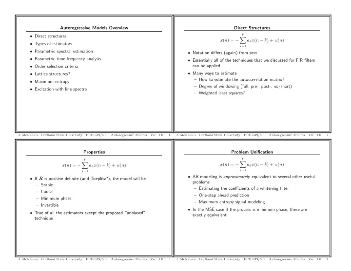
Autoregressive Models Overview Direct Structures P Direct - PowerPoint PPT Presentation

Autoregressive Models Overview Direct Structures P • Direct structures � x ( n ) = − a k x ( n − k ) + w ( n ) • Types of estimators k =1 • Parametric spectral estimation • Notation differs (again) from text • Parametric time-frequency analysis • Essentially all of the techniques that we discussed for FIR filters can be applied • Order selection criteria • Many ways to estimate • Lattice structures? – How to estimate the autocorrelation matrix? • Maximum entropy – Degree of windowing (full, pre-, post-, no/short) • Excitation with line spectra – Weighted least squares? J. McNames Portland State University ECE 539/639 Autoregressive Models Ver. 1.01 1 J. McNames Portland State University ECE 539/639 Autoregressive Models Ver. 1.01 2 Properties Problem Unification P P � � x ( n ) = − a k x ( n − k ) + w ( n ) x ( n ) = − a k x ( n − k ) + w ( n ) k =1 k =1 • AR modeling is approximately equivalent to several other useful • If ˆ R is positive definite (and Toeplitz?), the model will be problems – Stable – Estimating the coefficients of a whitening filter – Causal – One-step ahead prediction – Minimum phase – Maximum entropy signal modeling – Invertible • In the MSE case if the process is minimum phase, these are • True of all the estimators except the proposed “unbiased” exactly equivalent technique J. McNames Portland State University ECE 539/639 Autoregressive Models Ver. 1.01 3 J. McNames Portland State University ECE 539/639 Autoregressive Models Ver. 1.01 4

Windowing Autoregressive Estimation Windowing We have discussed three types of windowing • Parametric windowing is mostly reserved for nonstationary applications • Data Windowing : x w ( n ) = w ( n ) x ( n ) – Time-frequency analysis – Used to reduce spectral leakage of nonparametric PSD • Text seems to implicity suggest using data windowing estimators – This is a bad idea! • Correlation Windowing : r w ( ℓ ) = ˆ r ( ℓ ) w ( ℓ ) – Biases the estimate – Used to reduce variance of nonparametric PSD estimators – No obvious gain • Weighted Least Squares : E e = � N − 1 n =0 w 2 n | y ( n ) − c T x ( n ) | 2 • Is much better to perform a weighted least squares – Used to weight the influence of some observations more than – Each row of the data matrix and output still correspond to a others specific time – Optimal when error variance is non-constant in the – Estimate is unbiased deterministic data matrix case – Permits you to weight the influence of points near the center of the observation window (block) more heavily – Can be used with any non-negative window (need not be positive definite) J. McNames Portland State University ECE 539/639 Autoregressive Models Ver. 1.01 5 J. McNames Portland State University ECE 539/639 Autoregressive Models Ver. 1.01 6 Frequency Domain Representation of the Error Signal AR Spectral Estimation � π � π ∞ | X (e jω ) | 2 | e ( n ) | 2 = 1 H (e jω ) | 2 d ω = 1 x ( n ) = h ( n ) ∗ w ( n ) | X (e jω ) | 2 | ˆ A (e jω ) | 2 d ω � E = | ˆ 2 π 2 π = ˆ − π − π e ( n ) = ˆ w ( n ) h i ( n ) ∗ x ( n ) n = −∞ H i (e jω ) X (e jω ) = X (e jω ) • This means solving for the coefficients that minimize the error also E (e jω ) = ˆ minimize the integral of the ratio of the ESDs ˆ H (e jω ) • Why can’t we just make ˆ H i (e jω ) large or ˆ A (e jω ) small at all ∞ � π | X (e jω ) | 2 = 1 � | e ( n ) | 2 E = H (e jω ) | 2 d ω frequencies? | ˆ 2 π − π n = −∞ � � – Recall the constraint a 0 = 1 in ˆ a = 1 ˆ a 1 . . . ˆ a P 1 � π � π • In the AR case, H ( z ) = a k = 1 a 0 = 1 A ( z ) A (e jω ) e jωk d ω A (e jω ) d ω • Note the frequency domain equations only exist if the signals are 2 π 2 π − π − π energy signals – Thus A (e jω ) is constrained to have unit area – Segments of stationary processes • This means solving for the coefficients that minimize the error also minimize the integral of the ratio of the ESDs J. McNames Portland State University ECE 539/639 Autoregressive Models Ver. 1.01 7 J. McNames Portland State University ECE 539/639 Autoregressive Models Ver. 1.01 8

AR Spectral Estimation Properties Bias-Variance Tradeoff � π � π ∞ • The order of the parametric model is the key parameter that | X (e jω ) | 2 | e ( n ) | 2 = 1 H (e jω ) | 2 d ω = 1 | X (e jω ) | 2 | ˆ A (e jω ) | 2 d ω � E = controls the tradeoff between bias and variance | ˆ 2 π 2 π − π − π n = −∞ • P too large • The frequency domain representation of the error makes it clear – The variance is manifest differently than in nonparametric that the impact of the error across the full frequency range in estimators uniform – Spectrum may contain spurious speaks – There is no benefit to fitting lower or higher frequency ranges – Also possible for a single frequency component to be split into more accurately, in general distinct peaks • The regions where | X (e jω ) | > | ˆ H (e jω ) | contribute more to the • P too small total error – The error will be minimized if | ˆ – Insufficient peaks H (e jω ) | is larger in these regions – Peaks that are present are too wide or have the wrong shape – This is part of the reason the estimate is more accurate near spectral peaks, than valleys – Can only do so much with a pair of complex-conjugate poles – Nonparametric estimators were also more accurate near peaks, but for very different reasons (spectral leakage) J. McNames Portland State University ECE 539/639 Autoregressive Models Ver. 1.01 9 J. McNames Portland State University ECE 539/639 Autoregressive Models Ver. 1.01 10 Order Selection Problem Order Selection Methods Concept • There are many order selection criteria N f ˆ � 1 | e ( n ) | 2 Unbiased MSE u = • All try to obtain an approximately unbiased estimate of the MSE N f − N i +1 − P n = N i • All essentially add a penalty as the unscaled error increases N f ˆ 1 � | e ( n ) | 2 Biased MSE b = N f − N i +1 n = N i • Goal: Select the value of P that minimizes the MSE • We have two estimates of the MSE • One from Chapter 8 and one from Chapter 9 • The one from Chapter 8 was unbiased • Why don’t we use it to obtain the best value of P ? – Only holds in the deterministic data matrix case – The data matrix is always stochastic with AR models J. McNames Portland State University ECE 539/639 Autoregressive Models Ver. 1.01 11 J. McNames Portland State University ECE 539/639 Autoregressive Models Ver. 1.01 12

Possible Order Selection Methods Order Selection Methods Comments Let N t � N f − N i + 1 . Then • The order selection decision is only critical when P is on the same order as N t , say N t / 10 ≤ P < N t N f e � 1 – This is the difficult case of too little data to make a good σ 2 � | e ( n ) | 2 Model Error ˆ N t decision n = N i – None of the order selection criteria work good in this case FPE( P ) = N t + P σ 2 Final Prediction Error N t − P ˆ e • Otherwise σ 2 Akaike Information Criterion AIC( P ) = N t log ˆ e + 2 P – Similar performance will be obtained for a wide range of values of P σ 2 Minimum Description Length MDL( P ) = N t log ˆ e + P log N t – Can simply pick the value where the estimated parameter P CAT( P ) = 1 N t − k − N t − P vector stops changing with increasing values of P � Criterion Autoregressive Transfer σ 2 σ 2 N t N t ˆ N t ˆ e e • Text suggests looking at diagnostic plots (residuals, ACF, PACS, k =1 etc.) and selecting the parameter manually – Works well in many applications J. McNames Portland State University ECE 539/639 Autoregressive Models Ver. 1.01 13 J. McNames Portland State University ECE 539/639 Autoregressive Models Ver. 1.01 14 Maximum Entropy Motivation Maximum Entropy Problem • Suppose we know (i.e., have estimated) the autocorrelation of an • This discussion based on [1] WSS process for ℓ ≤ P • Suppose again that we have N observations of a random process • How do we extrapolate the estimated autocorrelation sequence for x ( n ) ℓ > P ? • If we knew the autocorrelation, we could calculate the AR • Let us denote the extrapolated values by r e ( ℓ ) parameters exactly (recall chapters 4 and 6) • Then the estimated PSD is given by • With only N observations, at most we can estimate r ( ℓ ) only for | ℓ | < N P R x (e jω = r x ( ℓ )e − jℓω + ˆ � � r e ( ℓ )e − jℓω • Many signals have autocorrelations that are non zero for ℓ ≥ N ℓ = − P | ℓ | >P • The segmentation may significantly impair the accuracy of the R x (e jω to have the same properties as a real PSD • We would like ˆ estimated parameters – Especially true of narrowband processes – Real-valued • Nonparametric PSD estimation methods simply extrapolate the – Nonnegative estimate r ( ℓ ) with zeros: ˆ r ( ℓ ) = 0 for ℓ ≥ N • These conditions are not sufficient for a unique extrapolation • Can we do better? • Need an additional constraint J. McNames Portland State University ECE 539/639 Autoregressive Models Ver. 1.01 15 J. McNames Portland State University ECE 539/639 Autoregressive Models Ver. 1.01 16