Time series of air pollutants Jiri Neubauer, Jaroslav Michalek, - PDF document

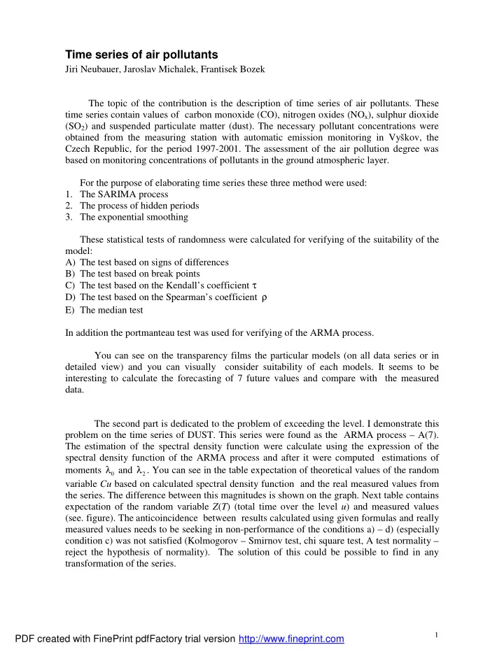
Time series of air pollutants Jiri Neubauer, Jaroslav Michalek, Frantisek Bozek The topic of the contribution is the description of time series of air pollutants. These time series contain values of carbon monoxide (CO), nitrogen oxides (NO x ), sulphur dioxide (SO 2 ) and suspended particulate matter (dust). The necessary pollutant concentrations were obtained from the measuring station with automatic emission monitoring in Vyškov, the Czech Republic, for the period 1997-2001. The assessment of the air pollution degree was based on monitoring concentrations of pollutants in the ground atmospheric layer. For the purpose of elaborating time series these three method were used: 1. The SARIMA process 2. The process of hidden periods 3. The exponential smoothing These statistical tests of randomness were calculated for verifying of the suitability of the model: A) The test based on signs of differences B) The test based on break points C) The test based on the Kendall’s coefficient τ D) The test based on the Spearman’s coefficient ρ E) The median test In addition the portmanteau test was used for verifying of the ARMA process. You can see on the transparency films the particular models (on all data series or in detailed view) and you can visually consider suitability of each models. It seems to be interesting to calculate the forecasting of 7 future values and compare with the measured data. The second part is dedicated to the problem of exceeding the level. I demonstrate this problem on the time series of DUST. This series were found as the ARMA process – A(7). The estimation of the spectral density function were calculate using the expression of the spectral density function of the ARMA process and after it were computed estimations of λ and λ . You can see in the table expectation of theoretical values of the random moments 0 2 variable Cu based on calculated spectral density function and the real measured values from the series. The difference between this magnitudes is shown on the graph. Next table contains expectation of the random variable Z ( T ) (total time over the level u ) and measured values (see. figure). The anticoincidence between results calculated using given formulas and really measured values needs to be seeking in non-performance of the conditions a) – d) (especially condition c) was not satisfied (Kolmogorov – Smirnov test, chi square test, A test normality – reject the hypothesis of normality). The solution of this could be possible to find in any transformation of the series. 1 PDF created with FinePrint pdfFactory trial version http://www.fineprint.com

For the future, it is counted on the development of a model which would enable to predict the concentration dependence of selected pollutants on temperature, pressure and humidity, air, wind intensity, inversion and other climate conditions. Further, the observation of the dependence of concentration development as for particular pollutants in interrelation and the attempt of possible determination of their synergetic or antagonistic effects is being considered. 2 PDF created with FinePrint pdfFactory trial version http://www.fineprint.com

ARIMA ARMA(p, q) Let { } ε be white noise, t = φ + φ + + φ + ε + θ ε + θ ε + + θ ε y y y ... y ... − − − − − − t 1 t 1 2 t 2 p t p t 1 t 1 2 t 2 q t q is a mixed autoregressive moving average process ARMA(p, q). = = = 2 Ly y , L ( Ly ) L y y In lag operator form ( ) − − t t 1 t t t 2 − φ − φ − − φ = + θ + θ + + θ ε 2 p 2 q ( 1 L L ... L ) y ( 1 L L ... L ) 1 2 p t 1 2 q t φ = θ ε ( L ) y ( L ) t t ARIMA(p, d, q) This model is convenient for description of nonstationary time series. ∆ = − = − = − y y y y Ly ( 1 L ) y 1-st difference … − t t t 1 t t t 2-nd difference … ∆ = ∆ ∆ = ∆ − = ∆ − ∆ = − + = 2 y ( y ) ( y y ) y y y 2 y y − − − − t t t t 1 t t 1 t t 1 t 2 = − + = − 2 2 ( 1 2 L L ) y ( 1 L ) y t t ARIMA(p, d, q) is defined as φ = θ ε ( L ) w ( L ) , t t where = ∆ d w y . t t We can write φ − = θ ε d ( L )( 1 L ) y ( L ) . t t SARIMA(p, d, q)(P, D, Q) lag s This model is convenient for description of nonstationary seasonal time series. = = = s s s 2 s L y y , L ( L y ) L y y The seasonal lag operator… − − t t s t t t 2 s ∆ = − s 1 L The seasonal difference operator … s ∆ = − = − s y ( 1 L ) y y y − s t t t t s ∆ = − = − + = − − + 2 s 2 s 2 s y ( 1 L ) y ( 1 2 L L ) y y 2 y y − s t t t t t s t 2 s We can write φ Φ − − = θ Θ ε s d s D s ( L ) ( L )( 1 L ) ( 1 L ) y ( L ) ( L ) . t t PDF created with FinePrint pdfFactory trial version http://www.fineprint.com

Properties of the autocorrelation function and the partial autocorrelation function and criteria AIC, FPE were used for determining the order of the model. Program STATISTICA and MATLAB were used for estimation of coefficients φ φ θ θ Φ Φ Θ Θ ,..., , ,..., , (Maximum likelihood estimation). ,..., , ,..., 1 p 1 q 1 P 1 Q Model of Hidden Periods Periodogram ( ω of time series y 1 , …, y n is defined as a function of variable ω The periodogram I ) ( ) 1 ω = ω + ω − π ≤ ω ≤ π 2 2 I ( ) a ( ) b ( ) , , π 4 where n 2 ∑ ω = ω a ( ) y cos( t ) , t n = t 1 n 2 ∑ ω = ω b ( ) y sin( t ) . t n = t 1 Using the periodogram we can find significant periods in time series y 1 , …, y n . We are trying to construct model of this series p ∑ = µ + α ω + β ω + ε = y ( cos( t ) sin t ) , t 1 ,..., n . t j j j j t = j 1 µ α j β ω are different are unknown parameters that is necessary to estimate, , , j j ω ∈ ( π ε is a normally distributed white noise ( σ 2 frequencies ( ), ). The 0 , ) N ( 0 , ) ε j t significant frequencies is possible to determine using a Fisher’s test. A null hypothesis in the Fisher test is = ε y , t t which suppose that series do not contains any significant periods. An alternative hypothesis supposes that there are some significant periods in this series. The Fisher’s test is based on values of the periodogram computing for frequencies π  −  2 j n 1 ω = = = * , j 1 ,..., m , m   j   n 2 High values of the periodogram determine significant frequencies. ω * I ( ) = j W max m = ∑ j 1 ,..., m ω * I ( ) j = i 1 The hull hypothesis is rejecting if W > g , F where g F is a critical value of the Fisher’s test (critical values are tabulated). PDF created with FinePrint pdfFactory trial version http://www.fineprint.com

µ α j β Parameters , , we can estimate using linear regression model j = Ax + ε y , t t t where [ ] = ω ω ω ω x 1 cos( t ) sin( t ) cos( t ) sin( t ) L , t 1 1 M M ω ,..., ω are significant frequencies, 1 M [ ] = µ α β α β A L . 1 1 M M Exponential Smoothing Brown’s Exponential Smoothing An exponential weights moving average is an average that weights the observed time series values unequally, with more recent observations being weighted more heavily than older observations. This unequal weighting is achieved through smoothing constants that determine how much weight is given to each observation. If m t-1 is the moving average calculated for the first t-1 points in the series y t then given the value y t , the new moving average is found as = α + − α m y ( 1 ) m , − t t t 1 <α < where α is the smoothing constant ( 0 1 ). For a data series y 1 , …, y n forecasts are given by = y m ˆ . − t t 1 The initial value m 0 is calculated as the average level in the first quarter of the series. Holt’s Linear Smoothing This adds a trend component to Brown’s Exponential method. For a data series y t forecasts are given by = − + y m b ˆ , − t t 1 t 1 where = α + − α − + m y ( 1 )( m b ) is the level at time t, − t t t 1 t 1 = γ − + − γ b ( m m ) ( 1 ) b is the trend at time t, − − t t t 1 t 1 <α < α is the level smoothing constant ( 0 1 ), < γ < γ is the trend smoothing constant ( 0 1 ). The initial values m 0 and b 0 are calculated by a linear regression on the first half of the series. PDF created with FinePrint pdfFactory trial version http://www.fineprint.com