Workshop 7.2a: Introduction to Linear models Murray Logan 19 Jul - - PowerPoint PPT Presentation

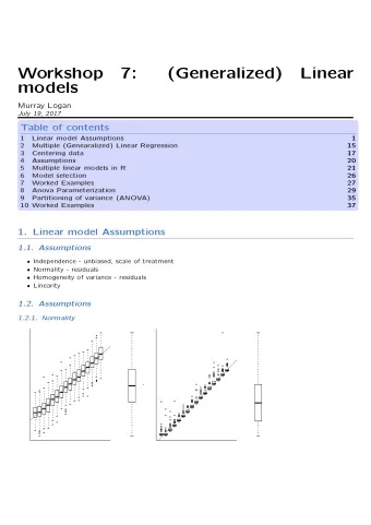
Workshop 7.2a: Introduction to Linear models

Murray Logan 19 Jul 2017

Section 1 Revision

Aims of statistical modelling

Use samples to:

• Describe relationships
• Inference testing (relationships/effects)
• Predictive models

Mathematical models

1 2 3 4 5 6

x

2 4 6 8 10 12

y

y = β0 + β1x

Statistical models

• 1

2 3 4 5 6

x

2 4 6 8 10 12

y

y = β0 + β1x + ε ε ~ Norm(0, σ2)

Linear models

• 1

2 3 4 5 6

x

2 4 6 8 10 12

y

y = β0 + β1x + ε

Linear models

• 1

2 3 4 5 6

x

20 40 60 80 100 120

y

y = β0 + β1x + β2x2

Non-linear models

• 1

2 3 4 5 6

x

500 1000 1500

y

y = αβx

Linear models

yi =

β0 + β1 ×

x1

+ ϵ1

response variable = population intercept

• intercept term

+ population

slope

× predictor

variable

• slope term
• Systematic component

+

error

Stoichastic component

Linear models

yi =

β0 + β1 ×

x1

+ ε1

response vector = intercept single value

• intercept term

+

slope single value × predictor vector

• slope term
• Systematic component

+

error

Stoichastic component

Vectors and Matrices

Vector Matrix

          3.0 2.5 6.0 5.5 9.0 8.6 12.0                     1 1 1 1 2 1 3 1 4 1 5 1 6          

Has length ONLY Has length AND width

Estimation

• 1

2 3 4 5 6

x

2 4 6 8 10 12

y

y = β0 + β1x + ε

Ordinary Least Squares

Estimation

Y X 3 2.5 1 6 2 5.5 3 9 4 8.6 5 12 6

3.0 = β0 × 1 + β1 × 0 + ε1 2.5 = β0 × 1 + β1 × 1 + ε1 6.0 = β0 × 1 + β1 × 2 + ε2 5.5 = β0 × 1 + β1 × 3 + ε3

Estimation

3.0 = β0 × 1 + β1 × 0 + ε1 2.5 = β0 × 1 + β1 × 1 + ε1 6.0 = β0 × 1 + β1 × 2 + ε2 5.5 = β0 × 1 + β1 × 3 + ε3 9.0 = β0 × 1 + β1 × 4 + ε4 8.6 = β0 × 1 + β1 × 5 + ε5 12.0 = β0 × 1 + β1 × 6 + ε6           3.0 2.5 6.0 5.5 9.0 8.6 12.0          

• Response values

=           1 1 1 1 2 1 3 1 4 1 5 1 6          

• Model matrix

× (β0 β1 )

Parameter vector

+         ε1 ε2 ε3 ε4 ε5 ε6        

• Residual vector

Inference testing

Ho:β1 = 0 (slope equals zero) The t-statistic t = param SEparam t = β1 SEβ1

Inference testing

Ho:β1 = 0 (slope equals zero) The t-statistic and the t distribution

Section 2 Linear model Assumptions

Assumptions

• Independence - unbiased, scale of

treatment

• Normality - residuals
• Homogeneity of variance - residuals
• Linearity

Assumptions

N

• r

m a l i t y

• y
• y

Assumptions

H

• m
• g

e n e i t y

• f

v a r i a n c e

• ●
• ●
• ●
• y

X Y

• ● ●
• ●
• x

y

• ●
• res

Predicted x Residuals

• ●
• ●
• ●
• y

X Y

• x

y

• res

Predicted x Residuals

Assumptions

L i n e a r i t y

Trendline

• 5

10 15 20 25 30 10 20 30 40 50 60

• 5

10 15 20 25 30 0.0 0.5 1.0 1.5 2.0 2.5

Assumptions

L i n e a r i t y

Loess (lowess) smoother

• 5

10 15 20 25 30 10 20 30 40 50 60

• 2.0

2.5

Assumptions

L i n e a r i t y

Spline smoother

• 5

10 15 20 25 30 10 20 30 40 50 60

• 5

10 15 20 25 30 0.0 0.5 1.0 1.5 2.0 2.5

Assumptions

yi = β0 + β1 × xi + εi

ϵi ∼ N(0, σ2)

Assumptions

yi = β0 + β1 × xi + εi

ϵi ∼ N(0, σ2)

Example

Make these data and call the data frame DATA Y X 3 2.5 1 6 2 5.5 3 9 4 8.6 5 12 6

Example

Make these data and call the data frame DATA Y X 3 2.5 1 6 2 5.5 3 9 4 8.6 5 12 6

• try this฀

> DATA <- data.frame(Y=c(3, 2.5, 6.0, 5.5, 9.0, 8.6, 12), X=0:6)

Worked Examples

> fert <- read.csv('../data/fertilizer.csv', strip.white=T) > fert FERTILIZER YIELD 1 25 84 2 50 80 3 75 90 4 100 154 5 125 148 6 150 169 7 175 206 8 200 244 9 225 212 10 250 248 > head(fert) FERTILIZER YIELD 1 25 84 2 50 80 3 75 90 4 100 154 5 125 148 6 150 169 > summary(fert) FERTILIZER YIELD Min. : 25.00 Min. : 80.0 1st Qu.: 81.25 1st Qu.:104.5 Median :137.50 Median :161.5 Mean :137.50 Mean :163.5 3rd Qu.:193.75 3rd Qu.:210.5 Max. :250.00 Max. :248.0 > str(fert) 'data.frame': 10 obs. of 2 variables: $ FERTILIZER: int 25 50 75 100 125 150 175 200 225 250 $ YIELD : int 84 80 90 154 148 169 206 244 212 248 > library(INLA) > > fert.inla <- inla(YIELD ~ FERTILIZER, data=fert) > summary(fert.inla)

Call: ฀inla(formula = YIELD ฀ FERTILIZER, data = fert)฀ Time used: Pre-processing Running inla Post-processing Total 0.3043 0.0715 0.0217 0.3974 Fixed effects: mean sd 0.025quant 0.5quant 0.975quant mode kld (Intercept) 51.9341 12.9747 25.9582 51.9335 77.8990 51.9339 0 FERTILIZER 0.8114 0.0836 0.6439 0.8114 0.9788 0.8114 0 The model has no random effects Model hyperparameters: mean sd 0.025quant 0.5quant 0.975quant mode Precision for the Gaussian observations 0.0035 0.0015 0.0012 0.0032 0.007 0.0028 Expected number of effective parameters(std dev): 2.00(0.00) Number of equivalent replicates : 5.00 Marginal log-Likelihood: -61.65

Worked Examples

Question: is there a relationship between fertilizer concentration and grass yeild? Linear model: Yi = β0 + β1Fi + εi

ε ∼ N(0, σ2)

Example

E x p l

• r

a t

• r

y d a t a a n a l y s i s

> library(car) > scatterplot(Y~X, data=DATA)

Example

E x p l

• r

a t

• r

y d a t a a n a l y s i s

> library(car) > peake <- read.csv('../data/peake.csv') > scatterplot(SPECIES ~ AREA, data=peake)

• 5000

Example

E x p l

• r

a t

• r

y d a t a a n a l y s i s

> scatterplot(SPECIES ~ AREA, data=peake, + smoother=gamLine)

• 5000

Example

E x p l

• r

a t

• r

y d a t a a n a l y s i s

> library(ggplot2) > library(gridExtra) > ggplot(peake, aes(y=SPECIES, x=AREA)) + geom_point()

• 5

> ggplot(peake, aes(y=SPECIES, x=AREA)) + geom_point() + + geom_smooth()

• 10

> p2 <- ggplot(peake, aes(y=SPECIES, x=1)) + geom_boxplot() > p3 <- ggplot(peake, aes(y=AREA, x=1)) + geom_boxplot() > grid.arrange(p1,p2,p3, ncol=3) Error in arrangeGrob(...): object 'p1' not found

Section 3 Simple Linear models in R

Linear models in R

> lm(formula, data= DATAFRAME)

Model R formula Description yi = β0 + β1xi

y~1+x y~x

Full model yi = β0

y~1

Null model yi = β1

y~-1+x

Through origin

Example

F i t l i n e a r m

• d

e l

yi = β0 + β1xi N(0, σ)

> DATA.lm<-lm(Y~X, data=DATA)

Worked Example

TIME TO FIT A MODEL

Linear models in R

Model diagnostics

R e s i d u a l s

• 1

2 3 4 5 6

x

5 10 15 20 25 30

y

Model diagnostics

R e s i d u a l s

• 1

2 3 4 5 6

x

5 10 15 20 25 30

y

Model diagnostics

L e v e r a g e

• 5

10 15 20

x

5 10 15 20 25 30

y

Model diagnostics

C

• k

’ s D

• 5

10 15 20

x

10 20 30 40 50

y

Example

M

• d

e l e v a l u a t i

• n

Extractor Description

residuals()

Extracts residuals from model

• 1

x

y

> residuals(DATA.lm) 1 2 3 4 5 6 7 0.8642857 -1.1428571 0.8500000 -1.1571429 0.8357143 -1.0714286 0.8214286

Example

M

• d

e l e v a l u a t i

• n

Extractor Description

residuals()

Extracts residuals from model

fitted()

Extracts the predicted values

• 1

x

y

> fitted(DATA.lm) 1 2 3 4 5 6 7 2.135714 3.642857 5.150000 6.657143 8.164286 9.671429 11.178571

Example

M

• d

e l e v a l u a t i

• n

Extractor Description

residuals()

Extracts residuals from model

fitted()

Extracts the predicted values

plot()

Series of diagnostic plots

> plot(DATA.lm)

• Residuals vs Fitted

• −1.0

Example

M

• d

e l e v a l u a t i

• n

Extractor Description

residuals()

Residuals

fitted()

Predicted values

plot()

Diagnostic plots

influence.measures()

Leverage (hat) and Cook฀s D

Example

M

• d

e l e v a l u a t i

• n

> influence.measures(DATA.lm) Influence measures of lm(formula = Y ~ X, data = DATA) : dfb.1_ dfb.X dffit cov.r cook.d hat inf 1 0.9603 -7.99e-01 0.960 1.82 0.4553 0.464 2 -0.7650 5.52e-01 -0.780 1.15 0.2756 0.286 3 0.3165 -1.63e-01 0.365 1.43 0.0720 0.179 4 -0.2513 -7.39e-17 -0.453 1.07 0.0981 0.143 5 0.0443 1.60e-01 0.357 1.45 0.0696 0.179 6 0.1402 -5.06e-01 -0.715 1.26 0.2422 0.286 7 -0.3466 7.50e-01 0.901 1.91 0.4113 0.464

Example

M

• d

e l e v a l u a t i

• n

Extractor Description

residuals()

Residuals

fitted()

Predicted values

plot()

Diagnostic plots

influence.measures()

Leverage, Cook฀s D

summary()

Summarizes important output from model

Example

M

• d

e l e v a l u a t i

• n

> summary(DATA.lm) Call: lm(formula = Y ~ X, data = DATA) Residuals: 1 2 3 4 5 6 7 0.8643 -1.1429 0.8500 -1.1571 0.8357 -1.0714 0.8214 Coefficients: Estimate Std. Error t value Pr(>|t|) (Intercept) 2.1357 0.7850 2.721 0.041737 * X 1.5071 0.2177 6.923 0.000965 ***

• Signif. codes:

0 '***' 0.001 '**' 0.01 '*' 0.05 '.' 0.1 ' ' 1 Residual standard error: 1.152 on 5 degrees of freedom Multiple R-squared: 0.9055, Adjusted R-squared: 0.8866 F-statistic: 47.92 on 1 and 5 DF, p-value: 0.0009648

Example

M

• d

e l e v a l u a t i

• n

Extractor Description

residuals()

Residuals

fitted()

Predicted values

plot()

Diagnostic plots

influence.measures()

Leverage, Cook฀s D

summary()

Model output

confint()

Confidence intervals of parameters

Example

M

• d

e l e v a l u a t i

• n

> confint(DATA.lm) 2.5 % 97.5 % (Intercept) 0.1178919 4.153537 X 0.9474996 2.066786

Example

M

• d

e l e v a l u a t i

• n

Extractor Description

residuals()

Residuals

fitted()

Predicted values

plot()

Diagnostic plots

influence.measures()

Leverage, Cook฀s D

summary()

Model output

confint()

Confidence intervals

predict()

Predict responses to new levels of predictors

Example

M

• d

e l e v a l u a t i

• n

> predict(DATA.lm, newdata=data.frame(X=c(2.5, 4.1)), + se=TRUE) $fit 1 2 5.903571 8.315000 $se.fit 1 2 0.4488222 0.4969340 $df [1] 5 $residual.scale [1] 1.152017 > predict(DATA.lm, newdata=data.frame(X=c(2.5, 4.1)), + interval='confidence') fit lwr upr 1 5.903571 4.749837 7.057306 2 8.315000 7.037591 9.592409

Example

M

• d

e l e v a l u a t i

• n

> predict(DATA.lm, newdata=data.frame(X=c(2.5, 4.1)), + interval='prediction') fit lwr upr 1 5.903571 2.725409 9.081734 2 8.315000 5.089881 11.540119

Prediction

          3.0 2.5 6.0 5.5 9.0 8.6 12.0          

• Response values

=           1 1 1 1 2 1 3 1 4 1 5 1 6          

• Model matrix

× (β0 β1 )

Parameter vector

+         ε1 ε2 ε3 ε4 ε5 ε6        

• Residual vector

          1 1 1 1 2 1 3 1 4 1 5 1 6          

• Model matrix

× (2.136 1.507 )

• Parameter vector

=           2.136 3.643 5.150 6.657 8.164 9.671 11.179          

• Predicted values vector

Example

M

• d

e l e v a l u a t i

• n

Extractor Description

residuals()

Residuals

fitted()

Predicted values

plot()

Diagnostic plots

influence.measures()

Leverage, Cook฀s D

summary()

Model output

confint()

Confidence intervals

predict()

Predict new responses

plot(allEffects())

Effects plots

Example

M

• d

e l e v a l u a t i

• n

> library(effects) > plot(allEffects(DATA.lm))

X effect plot

X Y

2 4 6 8 10 12 1 2 3 4 5 6

Section 4 Worked Examples

Worked Examples

> fert <- read.csv('../data/fertilizer.csv', strip.white=T) > fert FERTILIZER YIELD 1 25 84 2 50 80 3 75 90 4 100 154 5 125 148 6 150 169 7 175 206 8 200 244 9 225 212 10 250 248 > head(fert) FERTILIZER YIELD 1 25 84 2 50 80 3 75 90 4 100 154 5 125 148 6 150 169 > summary(fert) FERTILIZER YIELD Min. : 25.00 Min. : 80.0 1st Qu.: 81.25 1st Qu.:104.5 Median :137.50 Median :161.5 Mean :137.50 Mean :163.5 3rd Qu.:193.75 3rd Qu.:210.5 Max. :250.00 Max. :248.0 > str(fert) 'data.frame': 10 obs. of 2 variables: $ FERTILIZER: int 25 50 75 100 125 150 175 200 225 250 $ YIELD : int 84 80 90 154 148 169 206 244 212 248

Worked Examples

Question: is there a relationship between fertilizer concentration and grass yeild? Linear model: Y ∗ i = β ∗ 0 + β1Fi + εi

ε ∼ N(0, σ2)

Worked Examples

> peake <- read.csv('../data/peakquinn.csv', strip.white=T) > head(peake) AREA INDIV 1 516.00 18 2 469.06 60 3 462.25 57 4 938.60 100 5 1357.15 48 6 1773.66 118 > summary(peake) AREA INDIV Min. : 462.2 Min. : 18.0 1st Qu.: 1773.7 1st Qu.: 148.0 Median : 4451.7 Median : 338.0 Mean : 7802.0 Mean : 446.9 3rd Qu.: 9287.7 3rd Qu.: 632.0 Max. :27144.0 Max. :1402.0

Worked Examples

Question: is there a relationship between mussel clump area and number

• f individuals?

Linear model: Indivi = β0 + β1Areai + εi

ε ∼ N(0, σ2)

ln(Indivi) = β0 + β1ln(Areai) + εi

ε ∼ N(0, σ2)