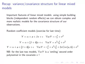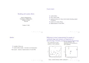
Outline Statistical inference for linear mixed models general form - PowerPoint PPT Presentation

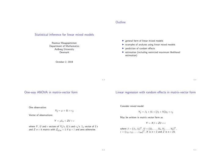
Outline Statistical inference for linear mixed models ◮ general form of linear mixed models Rasmus Waagepetersen ◮ examples of analyses using linear mixed models Department of Mathematics ◮ prediction of random effects Aalborg University ◮ estimation (including restricted maximum likelihood Denmark estimation) October 2, 2019 1 / 1 2 / 1 One-way ANOVA in matrix-vector form Linear regression with random effects in matrix-vector form Consider mixed model: One observation: Y ij = µ + U i + ǫ ij Y ij = β 1 + U i + [ β 2 + V i ] x ij + ǫ ij Vector of observations May be written in matrix vector form as Y = µ 1 n + ZU + ǫ Y = X β + ZU + ǫ where Y , U and ǫ vectors of Y ij ’s, U i ’s and ǫ ij ’s. 1 n vector of 1’s where β = ( β 1 , β 2 ) T , U = ( U 1 , . . . , U k , V 1 , . . . , V k ) T , and Z n × k matrix with Z ( ij ) q = 1 if q = i and zero otherwise. ǫ = ( ǫ 11 , ǫ 12 , . . . , ǫ km ) T , X is n × 2 and Z is n × 2 k . 3 / 1 4 / 1

Linear mixed model: general form Hierarchical version Consider model 1. U ∼ N (0 , Ψ) Y = X β + ZU + ǫ 2. Y | U = u ∼ N ( X β + Zu , Σ) where U ∼ N (0 , Ψ) and ǫ ∼ N (0 , Σ) are independent. Crucial assumption: Y normal given U ! All previous models special cases of this. Often Σ = σ 2 I so further assumption is individual observations Y i Then Y has multivariate normal distribution independent given U . Y ∼ N ( X β, Z Ψ Z T + Σ) Hierarchical version useful for extension to binary and count data. 5 / 1 6 / 1 Linear mixed models using lmer Linear mixed model for orthodont data - independent General lmer model formulation random slope and intercept y~‘fixed formula’+(‘rand formula_1’|Group_1)+ ... > ort6=lmer(distance~age*Sex+(1|Subject)+(-1+age|Subject)) +(‘rand. formula_n’|Group_n) > summary(ort6) translates into linear mixed model with independent sets of random Linear mixed model fit by REML effects for each grouping variable and e.g. Formula: distance ~ age * Sex + (1 | Subject) + (-1 + age | AIC BIC logLik deviance REMLdev (z|Group_i) 447.2 465.9 -216.6 428.1 433.2 corresponds to Random effects: U il + V il z Groups Name Variance Std.Dev. i.e. model with random intercept and random slope for covariate z Subject (Intercept) 2.4168043 1.554607 within each level l of grouping factor Group_i . Subject age 0.0077469 0.088017 Residual 1.8645950 1.365502 NB independence between levels of Group_i but intercept and Number of obs: 108, groups: Subject, 27 slope dependent within level. Fixed effects: Only random intercept respectively slope: (1|Group_i) resp. Estimate Std. Error t value (-1+z|Group_i) (Intercept) 16.34062 0.94087 17.368 7 / 1 8 / 1 age 0.78438 0.07944 9.874

Linear mixed model for orthodont data - correlated random Comparison of models for orthodont data slope and intercept Fixed part: age+Sex+age:sex > ort7=lmer(distance~age*Sex+(age|Subject)) Random part: > summary(ort7) Linear mixed model fit by REML Model AIC BIC logLik Number of parameters Formula: distance ~ age * Sex + (age | Subject) a 445.8 461.9 -216.9 4+2 AIC BIC logLik deviance REMLdev bx 448.7 464.8 -218.4 4+2 448.6 470 -216.3 427.9 432.6 a + bx , C ov ( a , b ) = 0 447.2 465.9 -216.6 4+3 Random effects: a + bx 448.6 470 -216.3 4+4 Groups Name Variance Std.Dev. Corr Subject (Intercept) 5.786427 2.40550 Larger logLik and smaller AIC or BIC means better model. age 0.032524 0.18035 -0.668 AIC and BIC takes into account number of parameters - penalizes Residual 1.716205 1.31004 complex models Number of obs: 108, groups: Subject, 27 The simplest one (just random intercept) seems better. Fixed effects: When REML (see last slide) is used (is default) for parameter Estimate Std. Error t value estimation, need same mean structure in the models compared. (Intercept) 16.3406 1.0185 16.043 9 / 1 10 / 1 age 0.7844 0.0860 9.121 SPSS SPSS - continued Choose Analyze → Mixed models → Linear. Need to specify ‘Subject’ variables - these correspond to the Under random: various options for covariance matrix of random grouping variables for lmer . effects within subject. Use covariance structure ’Variance Components’ to get independent random effects or ’unstructured’ With SPSS one can choose to model correlation in residuals to get dependent random effects. (Σ � = σ 2 I ) - then one also need to specify a ‘Repeated’ variable (e.g. residuals for each subject may be correlated in time). Remember to include intercept. Specify fixed part of model using item ‘fixed’ and random part Output: Type III F-tests for fixed effects. using item ‘random’ in menu. See also power-point slides regarding SPSS. Under random: several sets of random effects can be specified (corresponding to several (|) in R ). 11 / 1 12 / 1

Tests for fixed effects Nested two-way analysis of variance With lmer : to test the effect of a covariate or a factor you fit models with and without the covariate (or factor) and compute F-test using procedure KRmodcomp from pbkrtest package: > ort4=lmer(distance~age*Sex+(1|Subject)) For five cardboards we have 4 replications at 4 positions. > ort4.1=lmer(distance~age+Sex+(1|Subject))#remove interaction > library(pbkrtest) Hierarchical model (nested random effects) > KRmodcomp(ort4,ort4.1) F-test with Kenward-Roger approximation; computing time: 0.17 se Y ipj = µ + U i + U ip + ǫ ipj large : distance ~ age * Sex + (1 | Subject) small : distance ~ age + Sex + (1 | Subject) V ar Y ipj = τ 2 + ω 2 + σ 2 stat ndf ddf F.scaling p.value Ftest 6.3027 1.0000 79.0000 1 0.0141 * --- Signif. codes: 0 ’***’ 0.001 ’**’ 0.01 ’*’ 0.05 ’.’ 0.1 ’ ’ 1 Note: interaction now significant at 5% level. SPSS: F-tests available in output. 13 / 1 14 / 1 Covariance structure for nested random effects model Nested two-way analysis of variance > out2=lmer(Reflektans~(1|Pap.nr.)+(1|Pap.nr.*Sted)) > summary(out2) Y ipj = µ + U i + U ip + ǫ ipj Linear mixed model fit by REML AIC BIC logLik deviance REMLdev -432 -422.4 220 -443.8 -440  0 i � = l Random effects:    τ 2 Groups Name Variance Std.Dev.  i = l , p � = q same card  C ov ( Y ipj , Y lqk ) = τ 2 + ω 2 Pap.nr. (Intercept) 1.6560e-02 0.1286843 i = l , p = q same card and pos.   Pap.nr. * Sted (Intercept) 9.4539e-04 0.0307472 τ 2 + ω 2 + σ 2   i = 1 , p = q , k = j ( V ar Y ipj )  Residual 6.3494e-05 0.0079683 Number of obs: 80, groups: Pap.nr. * Sted, 20; Pap.nr., 5 Largest part of variance is between cardboard variance ! 15 / 1 16 / 1

A more complicated example: gene-expression Gene (DNA string) composed of substrings (exons) which may be more or less expressed according to treatment. Explanation of Reflektans~(1|Pap.nr.)+(1|Pap.nr.*Sted) : Expression measured as intensities on micro-array (chip). One chip ◮ no fixed formula: intercept always included as default pr. patient-treatment. ◮ (1|Pap.nr.) random intercepts for groups identified by variable Pap.nr. (card board effects) Factors: E (exon 8 levels), P (patient, 10 levels), T (treatment, 2 ◮ (1|Pap.nr.*Sted) random intercepts for groups identified levels) by cross of variables Pap.nr. and Sted (positions within cardboard) Y : vector of intensities (how much is exon expressed). ◮ random effects specified by different terms independent. Model: y ept = µ + α e + β t + γ et + U p + U pt + ǫ ept U pt and U p random chip and patient effects. Main question: are exons differentially expressed - i.e. are γ et � = 0 or not ? 17 / 1 18 / 1 Classical anova table: F-test for no treatment-exon interaction: 1.4278 with p -value 0.1998. > fit1=lm(intensity~treat*factor(exon)+factor(patient)+ factor(patient):treat,data=gene1) I.e. interaction not significant - no evidence of differential exon > anova(fit1) usage. Analysis of Variance Table Classical ANOVA: Response: intensity Df Sum Sq Mean Sq F value Pr(>F) ◮ not straightforward to obtain estimates of variance treat 1 3.242 3.242 14.4796 0.0002199 components from table of sums of squares (I will not go into factor(exon) 7 254.343 36.335 162.2852 < 2.2e-16 detail with this). factor(patient) 9 15.405 1.712 7.6449 6.703e-09 ◮ in the presence of random effects not straightforward to treat:factor(exon) 7 2.238 0.320 1.4278 0.1998234 compute F-tests for fixed effects (which sums of squares treat:factor(patient) 9 8.190 0.910 4.0643 0.0001345 should be used ?) Residuals 126 28.211 0.224 ◮ exact F-tests (only) available in balanced case (equal number σ 2 = 0 . 224 ˆ σ 2 of observations for each combination of factor levels) ˆ P × T = (0 . 91 − 0 . 224) / 8 = 0 . 08575 σ 2 ˆ P = (1 . 712 − 0 . 91) / 16 = 0 . 050125 19 / 1 20 / 1