Course topics Modeling with random effects random effects linear - PowerPoint PPT Presentation

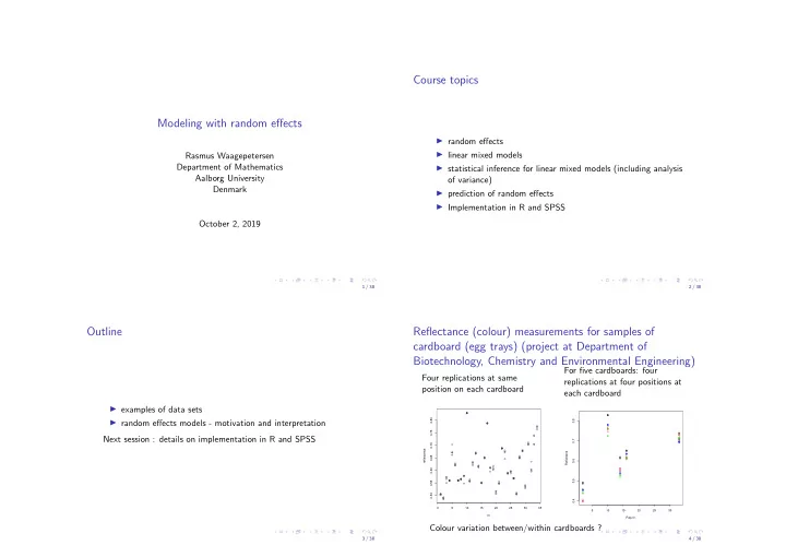
Course topics Modeling with random effects ◮ random effects ◮ linear mixed models Rasmus Waagepetersen Department of Mathematics ◮ statistical inference for linear mixed models (including analysis Aalborg University of variance) Denmark ◮ prediction of random effects ◮ Implementation in R and SPSS October 2, 2019 1 / 38 2 / 38 Outline Reflectance (colour) measurements for samples of cardboard (egg trays) (project at Department of Biotechnology, Chemistry and Environmental Engineering) For five cardboards: four Four replications at same replications at four positions at position on each cardboard each cardboard ◮ examples of data sets 0.80 ◮ random effects models - motivation and interpretation 0.8 0.75 Next session : details on implementation in R and SPSS 0.7 0.70 reflectance Reflektans 0.65 0.6 0.60 0.5 0.55 0.50 0.4 0 5 10 15 20 25 30 35 5 10 15 20 25 30 nr. Pap.nr. Colour variation between/within cardboards ? 3 / 38 4 / 38

Orthodontic growth curves (repeated Orthodontic growth curves (repeated measurements/longitudinal data) measurements/longitudinal data) Distance (related to jaw size) between pituitary gland and the Distance (related to jaw size) between pituitary gland and the pterygomaxillary fissure (two distinct points on human skull) for pterygomaxillary fissure (two distinct points on human skull) for children of age 8-14 children of age 8-14 Distance versus age grouped Distance versus age: Distance versus age: according to child 30 30 30 25 25 distance distance 25 distance 20 20 20 8 9 10 11 12 13 14 8 9 10 11 12 13 14 age age 8 9 10 11 12 13 14 age Different intercepts for different children ! 5 / 38 6 / 38 Model for reflectances: one-way anova Models: Y ij = µ + ǫ ij i = 1 , . . . , k j = 1 , . . . , m Four replications on each ( k = 34, m = 4) where µ Recall: basic aim for statistical analysis of a sample/dataset is to cardboard expectation and ǫ ij random extract information that can be generalized to the population that independent noise was sampled. 0.80 0.75 This perspective in mind when deciding on models for the datasets 0.70 considered. reflectance 0.65 0.60 0.55 0.50 0 5 10 15 20 25 30 35 nr. 7 / 38 8 / 38

Model for reflectances: one-way anova Model for reflectances: one-way anova Models: Models: Y ij = µ + ǫ ij i = 1 , . . . , k j = 1 , . . . , m Y ij = µ + ǫ ij i = 1 , . . . , k j = 1 , . . . , m Four replications on each Four replications on each ( k = 34, m = 4) where µ ( k = 34, m = 4) where µ cardboard cardboard expectation and ǫ ij random expectation and ǫ ij random independent noise or independent noise or 0.80 0.80 Y ij = µ + α i + ǫ ij Y ij = µ + α i + ǫ ij 0.75 0.75 0.70 0.70 reflectance where α i are fixed unknown reflectance where α i are fixed unknown 0.65 0.65 parameters parameters or 0.60 0.60 0.55 0.55 Y ij = µ + U i + ǫ ij 0.50 0.50 where U i are zero-mean random 0 5 10 15 20 25 30 35 0 5 10 15 20 25 30 35 nr. nr. variables independent of each other and of ǫ ij Which is most relevant ? 9 / 38 10 / 38 One role of random effects: parsimonious and population Second role of random effects: quantify sources of variation relevant models Quantify sources of variation (e.g. quality control): is pulp for paper production too heterogeneous ? With fixed effects α i : many parameters ( µ , σ 2 , α 2 , . . . , α 34 ). With random effects model Parameters α 2 , . . . , α 34 not interesting as they just represent intercepts for specific card boards which are individually not of Y ij = µ + U i + ǫ ij interest. we have decomposition of variance: With random effects: just three parameters ( µ , σ 2 = V ar ǫ ij and τ 2 = V ar U i ). V ar Y ij = V ar U i + V ar ǫ ij = τ 2 + σ 2 Hence parsimonious model. Variance parameters interesting for several reasons. Hence we can quantify variation between ( τ 2 ) cardboard pieces and within ( σ 2 ) cardboard. 11 / 38 12 / 38

Third role: modeling of covariance and correlation Covariances: Ratio γ = τ 2 /σ 2 is ‘signal to noise’.  0 i � = i ′   C ov [ Y ij , Y i ′ j ′ ] = i = i ′ , j � = j ′ V ar U i Proportion of variance  V ar U i + V ar ǫ ij i = i ′ , j = j ′  τ 2 γ σ 2 + τ 2 = γ + 1 Correlations:  is called intra-class correlation . 0 i � = i ′   τ 2 / ( σ 2 + τ 2 ) C orr [ Y ij , Y i ′ j ′ ] = i = i ′ , j � = j ′ High proportion of between cardboard variance leads to high  1 i = i ′ , j = j ′  correlation (next slide). That is, observations for same cardboard are correlated ! Correct modeling of correlation is important for correct evaluation of uncertainty. 13 / 38 14 / 38 Fourth role: correct evalution of uncertainty Classical balanced one-way ANOVA (analysis of variance) Suppose we wish to estimate µ = E Y ij . Due to correlation, Decomposition of empirical variance/sums of squares ( i = 1 , . . . , k , observations on same cardboard to some extent redundant. j = 1 , . . . , m ): µ = ¯ Y ·· . Evaluation of V ar ¯ Estimate is empirical average ˆ Y ·· : Y ·· ) 2 = Y ·· ) 2 = SSE + SSB � ( Y ij − ¯ � ( Y ij − ¯ � ( ¯ Y i · − ¯ Y i · ) 2 + m SST = Model erroneously ignoring Correct model with random ij ij i variation between cardboards cardboard effects Expected sums of squares: Y ij = µ + ǫ ij Y ij = µ + U i + ǫ ij , E SSE = k ( m − 1) σ 2 = σ 2 + τ 2 � V ar ǫ ij = σ 2 � V ar U i = τ 2 , V ar ǫ ij = σ 2 total E SSB = m ( k − 1) τ 2 + ( k − 1) σ 2 Naive variance expression is Correct variance expression is Moment-based estimates: = σ 2 + τ 2 Y ·· = σ 2 � � Y ·· = τ 2 k + σ 2 V ar ¯ total V ar ¯ σ 2 SSE τ 2 = SSB / ( k − 1) − ˆ σ 2 = n mk mk ˆ ˆ k ( m − 1) m With first model, variance is underestimated ! For V ar ¯ More complicated formulae in the unbalanced case. Y ·· → 0 is it enough that mk → ∞ ? 15 / 38 16 / 38

Hypothesis tests Classical implementation in R For cardboard/reflectance data, k = 34 and m = 4. anova() procedure produces table of sums of squares. Fixed effects: H 0 : α 1 = α 2 = · · · = α k > anova(lm(Reflektans~factor(Pap.nr.))) SSB / ( k − 1) F = Analysis of Variance Table SSE / ( k ( m − 1)) Response: Reflektans Random effects: H 0 : τ 2 = 0 Same test-statistic Df Sum Sq Mean Sq F value factor(Pap.nr) 33 0.9009 0.0273 470.7 #SSB SSB / ( k − 1) Residuals 102 0.0059 0.00006 #SSE F = SSE / ( k ( m − 1)) --- σ 2 = 0 . 00006, ˆ τ 2 = (0 . 0273 − 0 . 00006) / 4 = 0 . 00681. Idea: if τ 2 =0 then E SSB / ( k − 1) = E SSE / ( k ( m − 1)). Hence ˆ Biggest part of variation is between cardboard. 17 / 38 18 / 38 Orthodontic data: classical multiple linear regression in R Multiple linear regression continued - without interaction #fit model with sex specific intercepts and slopes > ort2=lm(distance~age+factor(Sex)) > ort1=lm(distance~age+age:factor(Sex)+factor(Sex)) > summary(ort1) Coefficients: Coefficients: Estimate Std. Error t value Pr(>|t|) Estimate Std. Error t value Pr(>|t|) (Intercept) 17.70671 1.11221 15.920 < 2e-16 *** (Intercept) 16.3406 1.4162 11.538 < 2e-16 *** age 0.66019 0.09776 6.753 8.25e-10 *** age 0.7844 0.1262 6.217 1.07e-08 *** factor(Sex)Female -2.32102 0.44489 -5.217 9.20e-07 *** factor(Sex)Female 1.0321 2.2188 0.465 0.643 age:factor(Sex)Female -0.3048 0.1977 -1.542 0.126 --- --- Signif. codes: 0 ’***’ 0.001 ’**’ 0.01 ’*’ 0.05 ’.’ 0.1 ’ Signif. codes: 0 ’***’ 0.001 ’**’ 0.01 ’*’ 0.05 ’.’ 0.1 ’ ’ 1 Residual standard error: 2.272 on 105 degrees of freedom Residual standard error: 2.257 on 104 degrees of freedom Multiple R-squared: 0.4095,Adjusted R-squared: 0.3983 Multiple R-squared: 0.4227,Adjusted R-squared: 0.4061 F-statistic: 36.41 on 2 and 105 DF, p-value: 9.726e-13 F-statistic: 25.39 on 3 and 104 DF, p-value: 2.108e-12 both age and sex significant Sex and age:Sex not significant ! 19 / 38 20 / 38