STAT 339 Hidden Markov Models III 21 April 2017 Bayesian - PowerPoint PPT Presentation

STAT 339 Hidden Markov Models III 21 April 2017 Bayesian Estimation / Model Averaging

Outline Inference Tasks in HMM Efficient Marginalization The Forward-Backward Algorithm Max Likelihood Parameter Estimation EM for HMMs EM Summary Gibbs Sampling for Model Averaging Model Averaging to Incorporate Uncertainty Gibbs Sampling to Draw from the Posterior Gibbs Summary Using the Samples

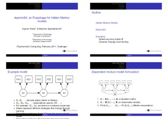
A Generative Model We can construct a generative model of the joint distribution of the z and the x p ( z , x ) = p ( z n ∣ z n − 1 ) p ( x n ∣ z n ) ∏ N n = 1 This corresponds to the graphical model below z 1 z 2 z n − 1 z n z n +1 x n − 1 x n +1 x 1 x 2 x n 3 / 35

Outline Inference Tasks in HMM Efficient Marginalization The Forward-Backward Algorithm Max Likelihood Parameter Estimation EM for HMMs EM Summary Gibbs Sampling for Model Averaging Model Averaging to Incorporate Uncertainty Gibbs Sampling to Draw from the Posterior Gibbs Summary Using the Samples 4 / 35

Inference in HMMs Given full specification of the component distributions (transition and emission probabilities), we might want to 1. Find the marginal distribution of a particular state p ( z n ′ ) or observation p ( x n ′ ) (e.g., predict the future or recover the past) Forward-Backward Algorithm 2. Evaluate marginal likelihood p ( x ) of some data (e.g., for model comparison) Forward Algorithm. 3. Find the most likely hidden sequence given data: argmax z p ( z ∣ x ) Viterbi Algorithm (we are skipping) 4. Get samples from p ( z ∣ x ) today 5 / 35

Learning HMMs n If we don’t know the transition and emission probabilities, we might want to 1. Find MLE transition matrix and emission parameters N p ( z n ∣ z n − 1 , A ) p ( x n ∣ z n , θ ) ∏ argmax A , θ n = 1 where the element A k,k ′ encodes p ( z n = k ′ , ∣ z n − 1 = k ) , and θ is a set of parameters of the “emission distributions” for each state. EM Algorithm 2. Do some model averaging using a posterior distribution over A and θ ; e.g., by getting samples A ( s ) , θ ( s ) ∼ p ( A , θ ∣ x ) MCMC (today) 6 / 35

Outline Inference Tasks in HMM Efficient Marginalization The Forward-Backward Algorithm Max Likelihood Parameter Estimation EM for HMMs EM Summary Gibbs Sampling for Model Averaging Model Averaging to Incorporate Uncertainty Gibbs Sampling to Draw from the Posterior Gibbs Summary Using the Samples 7 / 35

Outline Inference Tasks in HMM Efficient Marginalization The Forward-Backward Algorithm Max Likelihood Parameter Estimation EM for HMMs EM Summary Gibbs Sampling for Model Averaging Model Averaging to Incorporate Uncertainty Gibbs Sampling to Draw from the Posterior Gibbs Summary Using the Samples 8 / 35

Summary: Forward-Backward Algorithm We have defined the following shorthand: A ∶ transition matrix: a kk ′ ∶= p ( z n = k ′ ∣ z n − 1 = k ) B ∗ ∶ “observed” likelihood matrix: b ∗ nk ∶= p ( x n ∣ z n = k ) m n ∶ “cumulative” prior / “forward” message: m nk ∶= p ( z n = k,x 1 ∶ n ) r n ∶ “residual” likelihood / “backward” message: r nk ∶= p ( x n + 1 ∶ N ∣ z n = k ) We have also derived the following recursion formulas: m n = A T m n − 1 ⊙ b ∗ m 1 k = p ( z 1 = k ) p ( x 1 ∣ z 1 = k ) n , r n = A ⋅ ( b ∗ n + 1 ⊙ r n + 1 ) , r N = 1 9 / 35

Summary: Forward-Backward Algorithm We have defined the following shorthand: A ∶ transition matrix: a kk ′ ∶= p ( z n = k ′ ∣ z n − 1 = k ) B ∗ ∶ “observed” likelihood matrix: b ∗ nk ∶= p ( x n ∣ z n = k ) m n ∶ “cumulative” prior / “forward” message: m nk ∶= p ( z n = k,x 1 ∶ n ) r n ∶ “residual” likelihood / “backward” message: r nk ∶= p ( x n + 1 ∶ N ∣ z n = k ) Using these we can compute marginals for any n p ( z n ∣ x 1 ∶ N ) = p ( z n ,x 1 ∶ n ) p ( x n + 1 ∶ N ∣ z n ) = m n ⊙ r n p ( x 1 ∶ N ) m T n r n 9 / 35

Summary: Forward-Backward Algorithm We have defined the following shorthand: A ∶ transition matrix: a kk ′ ∶= p ( z n = k ′ ∣ z n − 1 = k ) B ∗ ∶ “observed” likelihood matrix: b ∗ nk ∶= p ( x n ∣ z n = k ) m n ∶ “cumulative” prior / “forward” message: m nk ∶= p ( z n = k,x 1 ∶ n ) r n ∶ “residual” likelihood / “backward” message: r nk ∶= p ( x n + 1 ∶ N ∣ z n = k ) As part of this calculation, we get the overall marginal likelihood of the model for free: p ( x 1 ∶ N ) = ∑ p ( z n = k,x 1 ∶ N ) = m T N 1 k 9 / 35

Outline Inference Tasks in HMM Efficient Marginalization The Forward-Backward Algorithm Max Likelihood Parameter Estimation EM for HMMs EM Summary Gibbs Sampling for Model Averaging Model Averaging to Incorporate Uncertainty Gibbs Sampling to Draw from the Posterior Gibbs Summary Using the Samples 10 / 35

Outline Inference Tasks in HMM Efficient Marginalization The Forward-Backward Algorithm Max Likelihood Parameter Estimation EM for HMMs EM Summary Gibbs Sampling for Model Averaging Model Averaging to Incorporate Uncertainty Gibbs Sampling to Draw from the Posterior Gibbs Summary Using the Samples 11 / 35

Maximum Likelihood Estimation ▸ We can parameterize the model using π kk ′ ∶ = p ( z n = k ′ ∣ z n − 1 = k, π ) f ( x ∣ θ k ) = p ( x ∣ z = k, θ ) ▸ Then we have a likelihood function for θ and π given z and data, x p ( z , x ∣ π , θ ) = ∏ N p ( z n ∣ z n − 1 ) p ( x n ∣ z n ) n = 1 = π z n − 1 z n f z n ( x n ∣ θ k ) ∏ N n = 1 = ( K K kk ′ )( K f k ( x n ∣ θ k )) ∏ ∏ ∏ ∏ π N kk ′ k = 1 k ′ = 1 k = 1 n ∶ z n = k where N kk ′ is the number of transitions from state k ′ to state k ′ in z 12 / 35

Max. Likelihood Estimation ▸ Then we have a likelihood function for θ and π given z and data, x p ( z , x ∣ π , θ ) = N p ( z n ∣ z n − 1 ) p ( x n ∣ z n ) ∏ n = 1 = ∏ N π z n − 1 z n f z n ( x n ∣ θ k ) n = 1 = ( kk ′ )( f k ( x n ∣ θ k )) ∏ K ∏ K ∏ K ∏ π N kk ′ k = 1 k ′ = 1 k = 1 n ∶ z n = k where N kk ′ is the number of transitions from state k ′ to state k ′ in z ▸ Factorizes into a piece with only π , and pieces with only one θ k each! ▸ Except this assumes we have z , which we don’t. 13 / 35

EM Returns! ▸ Fortunately, if we have a current guess about π and θ , then we can compute p ( z n = k ∣ x 1 ∶ N ) for each k ▸ Then simply assign each data point to every state, with weight q nk ∶ = p ( z n = k ∣ x 1 ∶ N ) ▸ We can compute these with forward-backward algorithm. 14 / 35

Quantum transitions ▸ To estimate π , need weights on possible transitions from n − 1 to n (for each ( k,k ′ ) pair) ▸ We want these weights to be ξ nkk ′ ∶ = p ( z n − 1 = k,z n = k ′ ∣ x 1 ∶ N ) ▸ We can write ξ nz n − 1 z n = p ( z n − 1 , x 1 ∶ n − 1 ) p ( z n ∣ z n − 1 ) p ( x n ∣ z n ) p ( x n + 1 ∶ N ∣ z n ) p ( x 1 ∶ N ) ξ nkk ′ = m n − 1 ,k a kk ′ b ∗ nk ′ r nk ′ m T N 1 15 / 35

Outline Inference Tasks in HMM Efficient Marginalization The Forward-Backward Algorithm Max Likelihood Parameter Estimation EM for HMMs EM Summary Gibbs Sampling for Model Averaging Model Averaging to Incorporate Uncertainty Gibbs Sampling to Draw from the Posterior Gibbs Summary Using the Samples 16 / 35

Summary: EM for HMMs We have developed the EM algorithm to do MLE of the HMM transition and emission parameters. 1. E-step: Execute forward-backward to compute the forward and backward messages, m 1 ,..., m N and r N ,..., r 1 , , and use them to compute weights q n ∶ = p ( z n ∣ x 1 ∶ N ) = m n ⊙ r n m T n r n ξ nkk ′ ∶ = p ( z n − 1 = k,z n = k ′ ∣ x 1 ∶ N ) = m n − 1 ,k a kk ′ b ∗ nk ′ r nk m T N 1 N kk ′ ∶ = ∑ ˜ ξ nkk ′ n 2. M-step: Maximize the “quantum” likelihood w.r.t π and θ ( kk ′ )( f k ( x n ∣ θ k ) q nk ) ∏ K ∏ K ∏ K ∏ ˜ N kk ′ π k = 1 k ′ = 1 k = 1 n 17 / 35

Outline Inference Tasks in HMM Efficient Marginalization The Forward-Backward Algorithm Max Likelihood Parameter Estimation EM for HMMs EM Summary Gibbs Sampling for Model Averaging Model Averaging to Incorporate Uncertainty Gibbs Sampling to Draw from the Posterior Gibbs Summary Using the Samples 18 / 35

Outline Inference Tasks in HMM Efficient Marginalization The Forward-Backward Algorithm Max Likelihood Parameter Estimation EM for HMMs EM Summary Gibbs Sampling for Model Averaging Model Averaging to Incorporate Uncertainty Gibbs Sampling to Draw from the Posterior Gibbs Summary Using the Samples 19 / 35

Maintaining Uncertainty ▸ As we’ve seen, MLE often does poorly unless we have a lot of data ▸ In particular if K is large compared to N , then we have K 2 parameters in π and some multiple of K in θ (where the multiple depends on complexity of each f k ( x ∣ θ k ) distribution) ▸ May not have too much precision to estimate π and θ . ▸ Also we really only have a local maximum. 20 / 35