Introduction to Hidden Markov Models Antonio Art es-Rodr guez - PowerPoint PPT Presentation

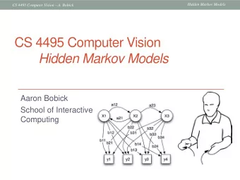
Introduction to Hidden Markov Models Antonio Art´ es-Rodr´ ıguez Unviersidad Carlos III de Madrid 2nd MLPM SS, September 17, 2014 1/33

Outline Markov and Hidden Markov Models Markov processes Definition of a HMM Applications of HMMs Inference in HMM Forward-Backward Algorithm Training the HMM Variations on HMMs From Gaussian to Mixture of Gaussian Emission Probabilities Incorporting Labels Autoregressive HMM Other Generalizations of HMMs Extensions on classical HMM methods Infinite Hidden Markov Model Spectral Learning of HMMs 2/33

Section 1 Markov and Hidden Markov Models 3/33

Markov processes Joint distribution of a sequence y 1: T p ( y 1: T ) = p ( y 1 ) p ( y 2 | y 1 ) . . . p ( y t | y 1: t − 1 ) . . . p ( y T | y 1: T − 1 ) ◮ First order Markov process p ( y 1: T ) = p ( y 1 ) p ( y 2 | y 1 ) . . . p ( y t | y t − 1 ) . . . p ( y T | y T − 1 ) y t − 1 y t y t +1 ◮ Second order Markov process p ( y 1: T ) = p ( y 1 ) p ( y 2 | y 1 ) . . . p ( y t | y t − 1 , y t − 2 ) . . . p ( y T | y T − 1 , y T − 2 ) ◮ First order homogeneous Markov process p ( y 2 | y 1 ) = · · · = p ( y t | y t − 1 ) = · · · = p ( y T | y T − 1 ) 4/33

Hidden Markov processes If the observed sequence y 1: T is a noisy version of the (first order) Markov process s 1: T p ( y 1: T , s 1: T ) = p ( y 1 | s 1 ) p ( s 1 ) . . . p ( y t | s t ) p ( s t | s t − 1 ) . . . . . . p ( y T | s T ) p ( s T | s T − 1 ) s t − 1 s t s t +1 y t − 1 y t y t +1 ◮ Discrete s t : Hidden Markov Model (HMM) ◮ Continuous s t : State Space Model (SSM) ◮ e.g. AR models 5/33

Coin Toss Example (from [Rabiner and Juang, 1986]) ◮ The result of tossing one-or-multiple fair-or-biased coins is y 1: T = hhttthtth · · · h ◮ Possible models: ◮ 1-coin model (not hidden): p ( y t = h | y t − 1 = h ) = p ( y t = h | y t − 1 = t ) = 1 − p ( y t = t | y t − 1 = h ) = 1 − p ( y t = t | y t − 1 = t ) ◮ 2-coin model: p ( y t = h | s t = 1) = p 1 p ( y t = t | s t = 1) = 1 − p 1 p ( y t = h | s t = 2) = p 2 p ( y t = t | s t = 2) = 1 − p 2 p ( s t = 1 | s t − 1 = 1) = a 11 p ( s t = 2 | s t − 1 = 1) = a 12 p ( s t = 1 | s t − 1 = 2) = a 21 p ( s t = 2 | s t − 1 = 2) = a 22 ◮ ... 6/33

The model s t − 1 s t s t +1 y t − 1 y t y t +1 ◮ S = { s 1 , s 2 , . . . , s T : s t ∈ 1 , . . . , I } : hidden state sequence. ◮ Y = { y 1 , y 2 , . . . , y T : y t ∈ R M } : observed continuous sequence ◮ A = { a ij : a ij = P ( s t +1 = j | s t = i ) } : state transition probabilities. ◮ B = { b i : P b i ( y t ) = P ( y t | s t = i ) } : observation emission probabilities. ◮ π = { π i : π i = P ( s 1 = i ) } : initial state probability distribution. ◮ θ = { A , B , π } : model parameters. 7/33

Applications of HMMs ◮ Automatic speech recognition ◮ s corresponds to phonemes or words and y to features extracted from the speech signal ◮ Activity recognition ◮ s corresponds to activities or gestures and y to features extracted from video or sensors signals ◮ Gene finding ◮ s corresponds to the location of the gene and y to DNA nucleotides ◮ Protein sequence alignment ◮ s corresponds to the matching to the latent consensus sequence and y to aminoacids 8/33

Section 2 Inference in HMM 9/33

Three Inference Problems for HMMs Problem 1: Given Y and θ , determine p ( Y | θ ). � O ( I T ) p ( Y | θ ) = p ( Y , S | θ ) S s T p ( Y , s T | θ ) ( O ( I 2 T )) (Forward ◮ p ( Y | θ ) = � algorithm) Problem 2: Given Y and θ , determine the “optimal” S . ◮ p ( s t | Y , θ ) ( O ( I 2 T )) (Forward-Backward algorithm) p ( Y | S , θ ) ( O ( I 2 T )) (Viterbi algorithm) ◮ argmax S Problem 3: Determine θ to maximize p ( Y | θ ). 10/33

Forward-Backward Algorithm P ( Y , s t = i ) P ( s t = i | Y ) = γ t ( i ) = P ( Y ) P ( y t +1: T | s t = i ) P ( y 1: t , s t = i ) = P ( Y ) β t ( i ) α t ( i ) = P ( Y ) ◮ Forward: ◮ α 1 ( i ) = π i P b i ( y 1 ) 1 ≤ i ≤ I �� I � ◮ α t ( i ) = j =1 α t − 1 ( j ) a ji P b i ( y t ) 1 ≤ i ≤ I , 1 < t ≤ T 11/33

Forward-Backward Algorithm P ( Y , s t = i ) P ( s t = i | Y ) = γ t ( i ) = P ( Y ) P ( y t +1: T | s t = i ) P ( y 1: t , s t = i ) = P ( Y ) β t ( i ) α t ( i ) = P ( Y ) ◮ Forward: ◮ α 1 ( i ) = π i P b i ( y 1 ) 1 ≤ i ≤ I �� I � ◮ α t ( i ) = j =1 α t − 1 ( j ) a ji P b i ( y t ) 1 ≤ i ≤ I , 1 < t ≤ T ◮ Backward: ◮ β T ( i ) = 1 1 ≤ i ≤ I ◮ β t ( i ) = � I j =1 a ij P b j ( y t +1 ) β t +1 ( j ) 1 ≤ i ≤ I , 1 ≤ t < T 11/33

Third Inference Problem Joint distribution of S and Y and log-likelihood for N sequences     N T n T n �  p ( s n � p ( s n t | s n � p ( y n t | s n p ( S , Y ) = 1 ) t − 1 ) t )    n =1 t =2 t =1 ◮ EM (Baum-Welch) [Baum et al., 1970] ◮ Bayesian inference methods: ◮ Gibbs sampler [Robert et al., 1993] ◮ Variational Bayes [MacKay, 1997] 12/33

Baum-Welch (EM) Algorithm Joint distribution of S and Y and log-likelihood for N sequences     N T n T n �  p ( s n � p ( s n t | s n � p ( y n t | s n p ( S , Y ) = 1 ) t − 1 ) t )    n =1 t =2 t =1 N I � � � I ( s n log p ( S , Y | θ ) = 1 = i | Y , θ ) log π i + n =1 i =1 T n I I T n I � � � � I ( s n t − 1 = i , s n � � I ( s n t = i | Y , θ ) log p ( y n t = j | Y , θ ) log a ij + t | b i ) t =2 i =1 j =1 t =1 i =1 � N I � � � I ( s n = 1 = i | Y , θ ) log π i i =1 n =1 � N T n � I I � � � � I ( s n t − 1 = i , s n + t = j | Y , θ ) log a ij i =1 j =1 n =1 t =2 � N I T n � � � � I ( s n log p ( y n + t = i | Y , θ ) t | b i ) i =1 n =1 t =1 13/33

Baum-Welch (EM) Algorithm (II) � N I � � � I ( s n log p ( S , Y | θ ) = 1 = i | Y , θ ) log π i i =1 n =1   I I N T n � � � � I ( s n t − 1 = i , s n  log a ij + t = j | Y , θ )  i =1 j =1 n =1 t =2   I N T n � � � I ( s n  log p ( y n + t = i | Y , θ ) t | b i )  i =1 n =1 t =1 E step �� N � = � N n =1 I ( s n ◮ E 1 = i | Y , θ ) n =1 γ n , 1 ( i ) �� N � � T n � T n t =2 I ( s n t − 1 = i , s n = � N ◮ E t = j | Y , θ ) t =2 ξ n , t ( i , j ) n =1 n =1 �� N � � T n t =1 I ( s n = � N � T n ◮ E t = i | Y , θ ) t =1 γ n , t ( i ) n =1 n =1 ξ n , t ( i , j ) = P ( s n t − 1 = i , s n t = j | Y ) = α t ( i ) a ij P b j ( y t +1 ) β t +1 ( j ) 14/33

Baum-Welch (EM) Algorithm (III) � N I � � � I ( s n log p ( S , Y | θ ) = 1 = i | Y , θ ) log π i i =1 n =1 � N T n � I I � � � � I ( s n t − 1 = i , s n + t = j | Y , θ ) log a ij i =1 j =1 n =1 t =2 � N I T n � � � � I ( s n log p ( y n + t = i | Y , θ ) t | b i ) i =1 n =1 t =1 M step �� N � ◮ ˆ π i = n =1 γ n , 1 ( i ) / N �� N � �� I � � T n � N � T n ◮ ˆ a ij = t =2 ξ n , t ( i , j ) / t =2 ξ n , t ( i , j ) n =1 j =1 n =1 ◮ Gaussian emission probabilities: �� N � �� N � � T n � T n ◮ ˆ t =1 γ n , t ( i ) y n µ i = / t =1 γ n , t ( i ) n =1 t n =1 ∗ − � N � N � T n � T n t =1 γ n , t ( i ) y n t y n t =1 γ n , t ( i ) ˆ µ i ˆ µ ∗ ◮ ˆ t i n =1 n =1 Σ i = � N � T n t =1 γ n , t ( i ) n =1 15/33

Bayesian Inference Methods for HMM ◮ Priors: ◮ Independent Dirichlet distributions on the rows of A , a i = [ a i 1 · · · a iI ] ◮ If possible, conjugate priors on emission probability parameters: Dirichlet for discrete observations, Normal-Invert Wishart for Gaussian observations, ... 16/33

Bayesian Inference Methods for HMM ◮ Priors: ◮ Independent Dirichlet distributions on the rows of A , a i = [ a i 1 · · · a iI ] ◮ If possible, conjugate priors on emission probability parameters: Dirichlet for discrete observations, Normal-Invert Wishart for Gaussian observations, ... ◮ Inference methods ◮ Gibbs sampler: iterative sampling from { p ( s t | Y , S − t , θ ) : t = 1 , . . . , T } , p ( A | S ), p ( B | Y , S ), p ( π | S ) ◮ Samples from { p ( s t | Y , S − t , θ ) : t = 1 , . . . , T } can be efficiently generated using the Forward-Filtering Backward-Sampling (FF-BS) algorithm [Fr¨ uhwirth-Schnatter, 2006] ◮ Variational Bayes: maximization of the Evidence Lower BOund (ELBO) obtained by assuming independence among S , A , B , and π 16/33

Section 3 Variations on HMMs 17/33

From Gaussian to Mixture of Gaussian Emission Probabilities K K t | µ ik , Σ ik ) z n log p ( y n � N ( y n t = � z n t log N ( y n t | b i ) = log t | µ ik , Σ ik ) k =1 k =1   I N T n � � � I ( s n  log p ( y n t = i | Y , θ ) t | b i ) =  i =1 n =1 t =1   I K N T n � � � � I ( s n t = i | Y , θ ) I ( z n t = k | y n  log N ( y n t , θ ) t | µ ik , Σ ik )  i =1 k =1 n =1 t =1 E step � N T n � � � I ( s n t = i | Y , θ ) I ( z n t = k | y n E t , θ ) ∝ n =1 t =1 N T n N T n t | µ ik , Σ ik ) . � � � � γ n , t ( i ) c ik N ( y n = γ n , t ( i , k ) n =1 t =1 n =1 t =1 18/33