2 Forward Elimination Factored Portion Factored Portion - PowerPoint PPT Presentation

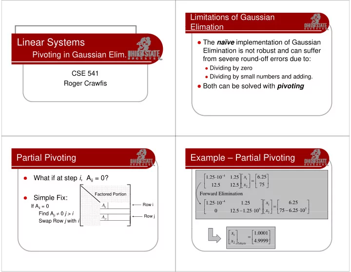
Limitations of Gaussian Elimation Elimation Linear Systems Linear Systems � The naïve implementation of Gaussian � The naïve implementation of Gaussian Elimination is not robust and can suffer Pivoting in Gaussian Elim. from severe round-off errors due to: from severe round off errors due to: � Dividing by zero CSE 541 � Dividing by small numbers and adding � Dividing by small numbers and adding. Roger Crawfis � Both can be solved with pivoting Partial Pivoting g Example – Partial Pivoting p g ⎡ ⎡ − ⎤ ⎤ ⋅ ⎡ ⎡ ⎤ ⎤ ⎡ ⎡ ⎤ ⎤ 4 x 6 . 25 � � What if at step i , A ii = 0? What if at step i A ii = 0? 1 . . 25 5 10 0 1 . . 25 5 = 1 1 ⎢ ⎢ ⎥ ⎥ ⎢ ⎥ ⎢ ⎥ ⎣ ⎦ ⎣ 75 ⎦ ⎣ 12 . 5 12 . 5 ⎦ x ⎡ ⎤ 2 Forward Elimination Factored Portion Factored Portion ⎢ ⎢ ⎥ ⎥ � Si Simple Fix: l Fi ⎡ − ⎤ ⋅ ⎡ ⎤ ⎡ ⎤ 4 x 6 . 25 1 . 25 10 1 . 25 Row i = ⎢ ⎢ ⎥ ⎥ 1 A If A ii = 0 ⎢ ⎥ ⎢ ⎥ ⎢ ⎥ ii − ⋅ − ⋅ 5 5 ⎣ ⎣ ⎦ ⎦ ⎣ ⎣ 75 75 6 6 . . 25 25 10 10 ⎦ ⎦ ⎣ ⎣ 0 0 12 12 . . 5 5 1 1 . . 25 25 10 10 ⎦ ⎦ x x Find A ji ≠ 0 j > i 2 2 Fi d A 0 j i ⎢ ⎥ Row j ⎣ A ⎦ ji Swap Row j with i ⎡ ⎤ ⎡ ⎤ 1 . 0001 x = 1 ⎢ ⎥ ⎢ ⎥ ⎣ x ⎦ ⎣ 4 . 9999 ⎦ 2 5 digits

Example – Partial Pivoting p g Better Pivoting g ⎡ − ⎤ ⋅ ⎡ ⎤ ⎡ ⎤ 4 1 . 25 10 1 . 25 x 6 . 25 ⎡ ⎡ ⎤ ⎤ ⎡ ⎡ ⎤ ⎤ � Partial Pivoting to mitigate round off error � Partial Pivoting to mitigate round-off error = = 1 1 . 0001 0001 1 x x ⎢ ⎢ ⎥ ⎥ ⎢ ⎢ ⎥ ⎥ ⎢ ⎢ ⎥ ⎥ = 1 ⎢ ⎥ ⎢ ⎥ ⎣ ⎦ ⎣ ⎦ ⎣ 75 ⎦ 12 . 5 12 . 5 x 2 ⎣ ⎦ ⎣ ⎦ x 4 . 9999 2 5 digits Forward Elimination If | | < max | | A A ii j ji > ⎡ ⎡ − ⎤ ⎤ ⋅ ⎡ ⎡ ⎤ ⎤ ⎡ ⎡ ⎤ ⎤ 4 4 j i j i 1 . 25 10 1 . 25 x 6 . 25 = 1 ⎢ ⎥ ⎢ ⎥ ⎢ ⎥ − ⋅ − ⋅ 5 5 ⎣ ⎦ ⎣ ⎦ ⎣ 75 6 . 25 10 ⎦ 0 12 . 5 1 . 25 10 x Swap row with arg (max | |) i A 2 ij > j j i Rounded to 3 digits Avoids Small ⎡ ⋅ − ⎤ ⎡ ⎤ ⎡ ⎤ 4 6 . 25 1 . 25 10 1 . 25 x = = 1 ⎢ ⎢ ⎥ ⎥ ⎢ ⎢ ⎥ ⎥ ⎢ ⎢ ⎥ ⎥ Multipliers Multipliers − ⋅ − ⋅ 5 5 ⎣ ⎦ ⎣ 6 . 25 10 ⎦ ⎣ 0 1 . 25 10 ⎦ x 2 � Adds an O ( n ) search. ⎡ ⎤ ⎡ ⎤ 0 x = 1 ⎢ ⎢ ⎥ ⎥ ⎢ ⎢ ⎥ ⎥ ⎣ ⎣ x ⎦ ⎦ ⎣ ⎣ 5 5 ⎦ ⎦ 2 3 digits Partial Pivoting g Pivoting strategies g g k swap � Partial Pivoting: � Partial Pivoting: ⎡ ⋅ − ⎤ ⎡ ⎤ ⎡ ⎤ 4 6 . 25 1 . 25 10 1 . 25 x = 1 1 ⎢ ⎢ ⎥ ⎥ ⎢ ⎢ ⎥ ⎥ ⎢ ⎢ ⎥ ⎥ ⎡ ⎤ ⎡ ⎤ ⎡ ⎤ 12 . 5 12 . 5 75 x k ⎣ 12 . 5 12 . 5 ⎦ ⎣ x ⎦ ⎣ 75 ⎦ 2 = 1 ⎢ ⎥ ⎢ ⎥ ⎢ ⎥ � Only row interchange ⋅ − 4 ⎣ 1 . 25 10 1 . 25 ⎦ ⎣ ⎦ ⎣ 6 . 25 ⎦ x 2 Forward Elimination Forward Elimination � Complete (Full) Pivoting � Complete (Full) Pivoting ⎡ ⎤ ⎡ ⎤ ⎡ ⎤ 12 . 5 12 . 5 x 75 k = 1 � Row and Column interchange ⎢ ⎥ ⎢ ⎥ ⎢ ⎥ − ⋅ − − ⋅ − 5 5 ⎣ ⎣ ⎦ ⎦ ⎣ ⎣ ⎦ ⎦ ⎣ ⎣ ⎦ ⎦ 0 1 . 25 12 . 5 10 x 6 . 25 75 10 2 2 � Threshold Pivoting k Rounded to 3 digits � Only if prospective pivot is found ⎡ ⎡ ⎤ ⎤ ⎡ ⎡ ⎤ ⎤ ⎡ ⎡ ⎤ ⎤ 12 12 . 5 5 12 12 . 5 5 75 75 x x 1 = to be smaller than a certain ⎢ ⎥ ⎢ ⎥ ⎢ ⎥ ⎣ 0 1 . 25 ⎦ ⎣ ⎦ ⎣ 6 . 25 ⎦ x 2 threshold ⎡ ⎡ ⎤ ⎤ ⎡ ⎡ ⎤ ⎤ 1 1 x = 1 ⎢ ⎥ ⎢ ⎥ ⎣ ⎦ ⎣ 5 ⎦ x 2 3 digits

Pivoting With Permutations g Pivoting � Adding permutation matrices in the mix: � Adding permutation matrices in the mix: � Again, the pivoting is strictly a function of � Again the pivoting is strictly a function of = the matrix A, so once we determine P it L L M P M P M P Ax M P M P M P b − − − − − − − − n 1 n 1 n 2 n 2 1 1 n 1 n 1 n 2 n 2 1 1 is trivial to apply it to many problems b k is trivial to apply it to many problems b k . � However, in Gaussian Elimination we will H i G i Eli i ti ill � For LU factorization we have: only swap rows or columns below the � LU = PA LU PA current pivot point. This implies a global t i t i t Thi i li l b l reordering of the equations will work: � Ly = Pb � Ux = y U = MPAx MPb ′ = ′ M A b