Stochastic Simulation Idea: probabilities samples Get probabilities - PowerPoint PPT Presentation

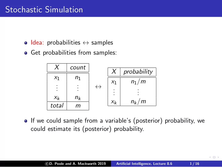
Stochastic Simulation Idea: probabilities ↔ samples Get probabilities from samples: X count X probability x 1 n 1 x 1 n 1 / m . . . . ↔ . . . . . . . . x k n k x k n k / m total m If we could sample from a variable’s (posterior) probability, we could estimate its (posterior) probability. � D. Poole and A. Mackworth 2019 c Artificial Intelligence, Lecture 8.6 1 / 16

Generating samples from a distribution For a variable X with a discrete domain or a (one-dimensional) real domain: Totally order the values of the domain of X . Generate the cumulative probability distribution: f ( x ) = P ( X ≤ x ). Select a value y uniformly in the range [0 , 1]. Select the x such that f ( x ) = y . � D. Poole and A. Mackworth 2019 c Artificial Intelligence, Lecture 8.6 2 / 16

Cumulative Distribution 1 1 P ( X ) f ( X ) 0 0 v 1 v 2 v 3 v 4 v 1 v 2 v 3 v 4 � D. Poole and A. Mackworth 2019 c Artificial Intelligence, Lecture 8.6 3 / 16

Hoeffding’s inequality Theorem (Hoeffding): Suppose p is the true probability, and s is the sample average from n independent samples; then P ( | s − p | > ǫ ) ≤ 2 e − 2 n ǫ 2 . Guarantees a probably approximately correct estimate of probability. � D. Poole and A. Mackworth 2019 c Artificial Intelligence, Lecture 8.6 4 / 16

Hoeffding’s inequality Theorem (Hoeffding): Suppose p is the true probability, and s is the sample average from n independent samples; then P ( | s − p | > ǫ ) ≤ 2 e − 2 n ǫ 2 . Guarantees a probably approximately correct estimate of probability. If you are willing to have an error greater than ǫ in δ of the cases, solve 2 e − 2 n ǫ 2 < δ for n , which gives � D. Poole and A. Mackworth 2019 c Artificial Intelligence, Lecture 8.6 4 / 16

Hoeffding’s inequality Theorem (Hoeffding): Suppose p is the true probability, and s is the sample average from n independent samples; then P ( | s − p | > ǫ ) ≤ 2 e − 2 n ǫ 2 . Guarantees a probably approximately correct estimate of probability. If you are willing to have an error greater than ǫ in δ of the cases, solve 2 e − 2 n ǫ 2 < δ for n , which gives n > − ln δ 2 2 ǫ 2 . � D. Poole and A. Mackworth 2019 c Artificial Intelligence, Lecture 8.6 4 / 16

Hoeffding’s inequality Theorem (Hoeffding): Suppose p is the true probability, and s is the sample average from n independent samples; then P ( | s − p | > ǫ ) ≤ 2 e − 2 n ǫ 2 . Guarantees a probably approximately correct estimate of probability. If you are willing to have an error greater than ǫ in δ of the cases, solve 2 e − 2 n ǫ 2 < δ for n , which gives n > − ln δ 2 2 ǫ 2 . ǫ δ n 0.1 0.05 185 0.01 0.05 18,445 0.1 0.01 265 � D. Poole and A. Mackworth 2019 c Artificial Intelligence, Lecture 8.6 4 / 16

Forward sampling in a belief network Sample the variables one at a time; sample parents of X before sampling X . Given values for the parents of X , sample from the probability of X given its parents. � D. Poole and A. Mackworth 2019 c Artificial Intelligence, Lecture 8.6 5 / 16

Rejection Sampling To estimate a posterior probability given evidence Y 1 = v 1 ∧ . . . ∧ Y j = v j : Reject any sample that assigns Y i to a value other than v i . The non-rejected samples are distributed according to the posterior probability: � = α 1 sample | P ( α | evidence ) ≈ � sample 1 where we consider only samples consistent with evidence. � D. Poole and A. Mackworth 2019 c Artificial Intelligence, Lecture 8.6 6 / 16

Rejection Sampling Example: P ( ta | sm , re ) Observe Sm = true , Re = true Ta Fi Al Sm Le Re s 1 false true false true false false Ta Fi Al Sm Le Re � D. Poole and A. Mackworth 2019 c Artificial Intelligence, Lecture 8.6 7 / 16

Rejection Sampling Example: P ( ta | sm , re ) Observe Sm = true , Re = true Ta Fi Al Sm Le Re s 1 false true false true false false ✘ s 2 false true true true true true Ta Fi Al Sm Le Re � D. Poole and A. Mackworth 2019 c Artificial Intelligence, Lecture 8.6 7 / 16

Rejection Sampling Example: P ( ta | sm , re ) Observe Sm = true , Re = true Ta Fi Al Sm Le Re s 1 false true false true false false ✘ s 2 false true true true true true ✔ Ta Fi s 3 true false true false Al Sm Le Re � D. Poole and A. Mackworth 2019 c Artificial Intelligence, Lecture 8.6 7 / 16

Rejection Sampling Example: P ( ta | sm , re ) Observe Sm = true , Re = true Ta Fi Al Sm Le Re s 1 false true false true false false ✘ s 2 false true true true true true ✔ Ta Fi s 3 true false true false — — ✘ s 4 true true true true true true Al Sm Le Re � D. Poole and A. Mackworth 2019 c Artificial Intelligence, Lecture 8.6 7 / 16

Rejection Sampling Example: P ( ta | sm , re ) Observe Sm = true , Re = true Ta Fi Al Sm Le Re s 1 false true false true false false ✘ s 2 false true true true true true ✔ Ta Fi s 3 true false true false — — ✘ s 4 true true true true true true ✔ . . . Al Sm s 1000 false false false false Le Re � D. Poole and A. Mackworth 2019 c Artificial Intelligence, Lecture 8.6 7 / 16

Rejection Sampling Example: P ( ta | sm , re ) Observe Sm = true , Re = true Ta Fi Al Sm Le Re s 1 false true false true false false ✘ s 2 false true true true true true ✔ Ta Fi s 3 true false true false — — ✘ s 4 true true true true true true ✔ . . . Al Sm s 1000 false false false false — — ✘ P ( sm ) = 0 . 02 Le P ( re | sm ) = 0 . 32 How many samples are rejected? Re How many samples are used? � D. Poole and A. Mackworth 2019 c Artificial Intelligence, Lecture 8.6 7 / 16

Importance Sampling Samples have weights: a real number associated with each sample that takes the evidence into account. Probability of a proposition is weighted average of samples: � = α weight ( sample ) sample | P ( α | evidence ) ≈ � sample weight ( sample ) Mix exact inference with sampling: don’t sample all of the variables, but weight each sample according to P ( evidence | sample ). � D. Poole and A. Mackworth 2019 c Artificial Intelligence, Lecture 8.6 8 / 16

Importance Sampling (Likelihood Weighting) procedure likelihood weighting ( Bn , e , Q , n ): ans [1 : k ] := 0 where k is size of dom ( Q ) repeat n times: weight := 1 for each variable X i in order: if X i = o i is observed weight := weight × P ( X i = o i | parents ( X i )) else assign X i a random sample of P ( X i | parents ( X i )) if Q has value v : ans [ v ] := ans [ v ] + weight return ans / � v ans [ v ] � D. Poole and A. Mackworth 2019 c Artificial Intelligence, Lecture 8.6 9 / 16

Importance Sampling Example: P ( ta | sm , re ) Ta Fi Al Le Weight s 1 true false true false Ta Fi s 2 false true false false s 3 false true true true s 4 true true true true Al Sm . . . s 1000 false false true true Le P ( sm | fi ) = 0 . 9 P ( sm | ¬ fi ) = 0 . 01 P ( re | le ) = 0 . 75 Re P ( re | ¬ le ) = 0 . 01 � D. Poole and A. Mackworth 2019 c Artificial Intelligence, Lecture 8.6 10 / 16

Importance Sampling Example: P ( ta | sm , re ) Ta Fi Al Le Weight s 1 true false true false 0 . 01 × 0 . 01 Ta Fi s 2 false true false false 0 . 9 × 0 . 01 s 3 false true true true 0 . 9 × 0 . 75 s 4 true true true true 0 . 9 × 0 . 75 Al Sm . . . s 1000 false false true true 0 . 01 × 0 . 75 Le P ( sm | fi ) = 0 . 9 P ( sm | ¬ fi ) = 0 . 01 P ( re | le ) = 0 . 75 Re P ( re | ¬ le ) = 0 . 01 � D. Poole and A. Mackworth 2019 c Artificial Intelligence, Lecture 8.6 10 / 16

Importance Sampling Example: P ( le | sm , ta , ¬ re ) P ( ta ) = 0 . 02 P ( fi ) = 0 . 01 Ta Fi P ( al | fi ∧ ta ) = 0 . 5 P ( al | fi ∧ ¬ ta ) = 0 . 99 P ( al | ¬ fi ∧ ta ) = 0 . 85 Al Sm P ( al | ¬ fi ∧ ¬ ta ) = 0 . 0001 P ( sm | fi ) = 0 . 9 P ( sm | ¬ fi ) = 0 . 01 Le P ( le | al ) = 0 . 88 P ( le | ¬ al ) = 0 . 001 P ( re | le ) = 0 . 75 Re P ( re | ¬ le ) = 0 . 01 � D. Poole and A. Mackworth 2019 c Artificial Intelligence, Lecture 8.6 11 / 16

Computing Expectations & Proposal Distributions Expected value of f with respect to distribution P : � E P ( f ) = f ( w ) ∗ P ( w ) w � D. Poole and A. Mackworth 2019 c Artificial Intelligence, Lecture 8.6 12 / 16

Computing Expectations & Proposal Distributions Expected value of f with respect to distribution P : � E P ( f ) = f ( w ) ∗ P ( w ) w ≈ 1 � f ( s ) n s s is sampled with probability P . There are n samples. � D. Poole and A. Mackworth 2019 c Artificial Intelligence, Lecture 8.6 12 / 16

Computing Expectations & Proposal Distributions Expected value of f with respect to distribution P : � E P ( f ) = f ( w ) ∗ P ( w ) w ≈ 1 � f ( s ) n s s is sampled with probability P . There are n samples. � E P ( f ) = f ( w ) ∗ P ( w ) / Q ( w ) ∗ Q ( w ) w � D. Poole and A. Mackworth 2019 c Artificial Intelligence, Lecture 8.6 12 / 16