1 7 8 Types of simulation models Dynamic simulation models - PDF document
2 Outlines Simulation Modeling in Animal Health Management: Introduction: What is simulation modeling? A Stochastic Bio-economic Model of Bovine Intramammary Why simulation modeling is used? Infections (IMI) What are the
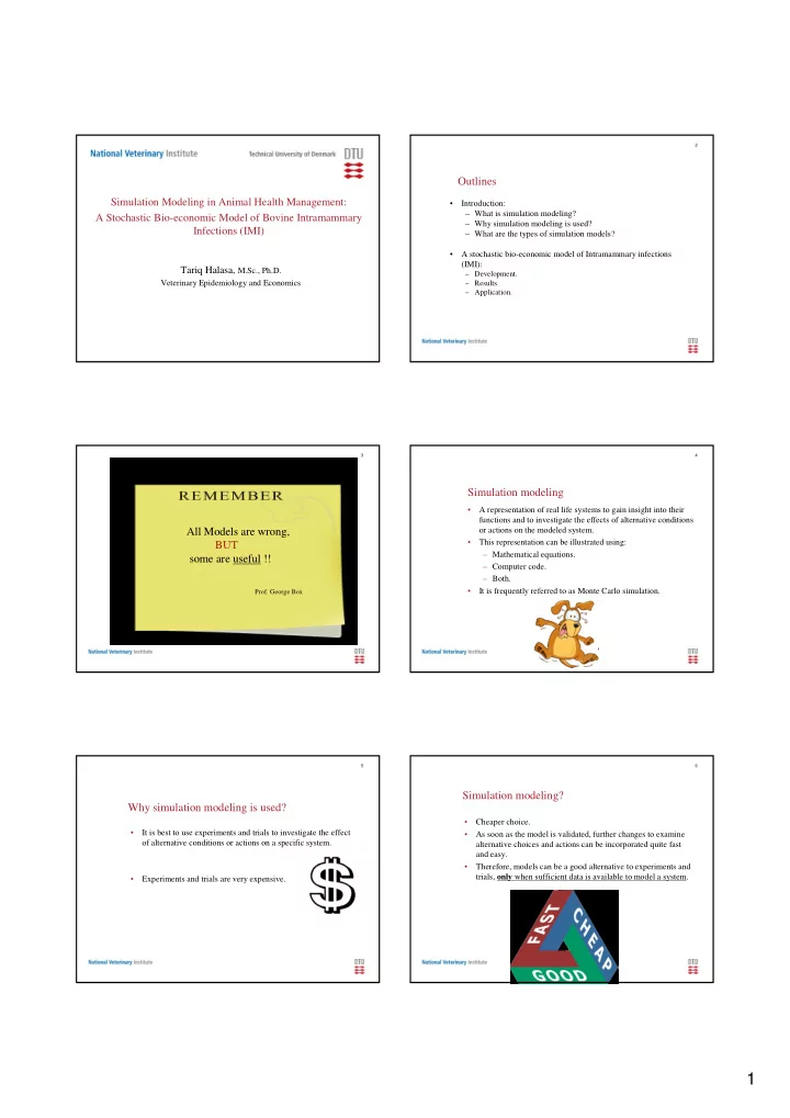
2 Outlines Simulation Modeling in Animal Health Management: • Introduction: – What is simulation modeling? A Stochastic Bio-economic Model of Bovine Intramammary – Why simulation modeling is used? Infections (IMI) – What are the types of simulation models? • A stochastic bio-economic model of Intramammary infections (IMI): Tariq Halasa, M.Sc., Ph.D. – Development. Veterinary Epidemiology and Economics – Results. – Application. 3 4 Simulation modeling • A representation of real life systems to gain insight into their functions and to investigate the effects of alternative conditions or actions on the modeled system. All Models are wrong, • This representation can be illustrated using: BUT – Mathematical equations. some are useful !! – Computer code. – Both. • It is frequently referred to as Monte Carlo simulation. Prof. George Box 5 6 Simulation modeling? Why simulation modeling is used? • Cheaper choice. • It is best to use experiments and trials to investigate the effect • As soon as the model is validated, further changes to examine of alternative conditions or actions on a specific system. alternative choices and actions can be incorporated quite fast and easy. • Therefore, models can be a good alternative to experiments and trials, only when sufficient data is available to model a system. • Experiments and trials are very expensive. 1
7 8 Types of simulation models Dynamic simulation models • Stochastic vs. deterministic. • Continuous vs. discrete: – Deterministic: use one input value to represent the occurrence of – Continuous: based on continuous solving of differential an event; for instance the use of average values. equations. – Stochastic: use randomness to model chance or events; for – Discrete: chronological sequence of events occurring at instance the use of probability distribution. instant points in time and result in a change of state in the modeled system. A discrete time period can be a day, a • Static vs. dynamic. week, a month or a year… et cetera . – Dynamic: changes in the modeled system occur as response to changes over the course of time. – Static: the course of time is not modeled. 9 10 Intramammary infections ( IMI ) or mastitis • Intramammary infections ( IMI ) is “synonym” to mastitis, which is the inflammation of mammary glands. • It can be caused by different pathogens. A Stochastic Bio-economic Model of Bovine Intramammary • It leads to: Infections (IMI) – Adverse welfare effect, pain to the infected cow. – Economic damage to the farmer: milk production loss, use of antibiotics to treat the infected cow, and higher risk of culling the infected cow. • It is the costly endemic disease in the developed countries. Mastitis 11 12 A stochastic bio-economic model of bovine intramammary infections (IMI) • Bio-economics: the integration of economic analysis on the Mastitis course of a biological system to provide economic sound Mastitis decisions. • Stochastic dynamic discrete-event simulation model. • Each discrete time step is represented by 2-weeks. • Halasa et al. (2009), Livestock Science 124:295-305 . Healthy 2
13 14 Objectives Choice of modeling procedure • Simulate a herd of dairy cows to: • Obtain insight into the dynamics of pathogen-specific IMI over time and determine their effects on the variability of the costs – Obtain insight into the dynamics of pathogen-specific IMI in of IMI. Dutch bovine dairy herds to better prevent and control IMI. – Estimate the costs of IMI in an endemic situation in Dutch bovine • Investigate alternative actions to prevent and control pathogen- dairy herds. specific IMI. – Support decision making in relation to IMI prevention and control. • Predict economic consequences of future changes of IMI management. 15 16 Modeled IMI pathogens Contagious transmission of IMI pathogens Staphylococcus aureus • • An IMI cow transmits the infection to healthy herd mates through Streptococcus uberis Contagious pathogens • the milking process, equipments and the farmer. (Zadoks et al., 2001; 2002) Streptococcus dysgalactiae • Escherichia coli • Environmental pathogen 17 18 Modeling contagious IMI pathogens Environmental IMI • Reed-frost model: explains the infection behavior of a contagious • Infection originates from the environment. pathogen in a population of susceptible individuals. • The probability of new infections at a specific discrete point in time is dependent on: – The transmission rate parameter ( β ) of the IMI pathogen, which represent the average probability of new infection per unit of time. – The number of infectious animals (I). – The total number of lactating animals (N). Probability of infection = 1- EXP(- β * I * � T / N). � T is the time • difference. • The probability of infection is calculated by the model at each discrete time period. Therefore, it is dynamic. 3
19 20 Modeling IMI pathogens Modeling environmental IMI pathogen ( E. coli ) • Greenwood model: explains the infection behavior of a pathogen originates from the environment in a population of susceptible individuals. • The probability of infection at any point in time is independent from the number of infected animals; given that the pathogen exists in the environment permanently. • The probability of new infections at any point in time is based on: The cumulative incidence of E. coli IMI per 14 cow-days at risk. – • The probability of infection is fixed over the discrete time period of the model. Probability of infection in: - Contagious transmission = 1- EXP(- β * I * � T / N). - Environmental transmission = fixed value / 14-cow days. 21 22 Modeling the dynamics of IMI during the lactation Modeling the dynamics of IMI during the lactation Healthy (No IMI) 2 weeks 2 weeks The lactation The lactation 23 24 Modeling the dynamics of IMI during the lactation Modeling the dynamics of IMI during the lactation X Culled Clinical IMI (CIMI) Subclinical IMI (SCIMI) Healthy Healthy Healthy CIMI IMI IMI SCIMI 2 weeks 2 weeks The lactation The lactation 4
25 26 Modeling the dynamics of IMI during the lactation Modeling the dynamics of IMI during the lactation: X Culled State transition probabilities Healthy • State changing is based on probabilities: CIMI – Become a new IMI case. Healthy SCIMI – Cure from IMI. – Be culled. Healthy – Change the IMI status. IMI • These transitional probabilities are used in different random distributions SCIMI SCIMI to determine the state of each cow at each discrete time period. 2 weeks CIMI X Culled The lactation 27 28 Input parameters for the dynamics of IMI • Pathogen-specific transmission parameters obtained from field studies ( Zadoks et al., 2001; 2002 ). Any question • Other parameters obtained from field studies and experiments and were pathogen-specific. • All rates and probabilities were recalculated per 14 cow-days, because each discrete time period in the model was 14 days. Replacement ( α ) was based on • the quota situation. 29 30 Modeling the herd Modeling cow level production • The model simulates a herd of 100 dairy cattle within 1 quota- • Milk production per cow was calculated based on the lactation year. curve of wood (Wood et al., 1976). • The herd demography was based on Dutch data from the national recording system and from field studies. 30 – Distribution of age in the herd (parity numbers). 25 Milk production – Lactation stage and length. 20 – Milk production per cow. 15 • Several random distributions were used to determine the herd 10 demographical characteristics. 5 5 10 15 20 Time period 5
31 32 Effects of IMI on milk production Modeling cow level production • Mastitis or IMI results in decrease milk production. • Milk production loss due to clinical and subclinical IMI. – Clinical mastitis causes a persistent loss of milk production (Grohn et al., 2004). – Subclinical mastitis causes milk production loss (Halasa et al., IMI 2009). 30 25 Milk production 20 15 10 5 5 10 15 20 Time period 33 34 Modeling cow level production Modeling the herd level milk production and milk quota • Herd level milk production at time period t = • Milk production loss due to clinical and subclinical IMI. Σ (milk production of all cows at time period t). • Cumulative herd level milk production at time period t = IMI Σ (herd level milk production at time period t + t-1). 30 25 Milk production • Milk quota was defined as the total milk that should be produced within 1 year. 20 • IMI reduce milk production. So the quota might not be reached. 15 • What should the farmer do????? 10 5 5 10 15 20 Time period Economic effects 35 36 Modeling milk quota • Cumulative herd level milk production was calculated at each time period twice: – Including the effects of IMI (milk production loss) and culling. – Excluding the effects of IMI and culling (the total milk that should be produced to reach the quota by the end of the year). • Milk quota deficiency = cumulative herd level milk production excluding effects of IMI and culling - cumulative herd level milk production including effects of IMI and culling. When the milk quota deficiency ≥ a production of an average cow, a • new cow was included (replacement ( α )). 6
Recommend
More recommend
Explore More Topics
Stay informed with curated content and fresh updates.
