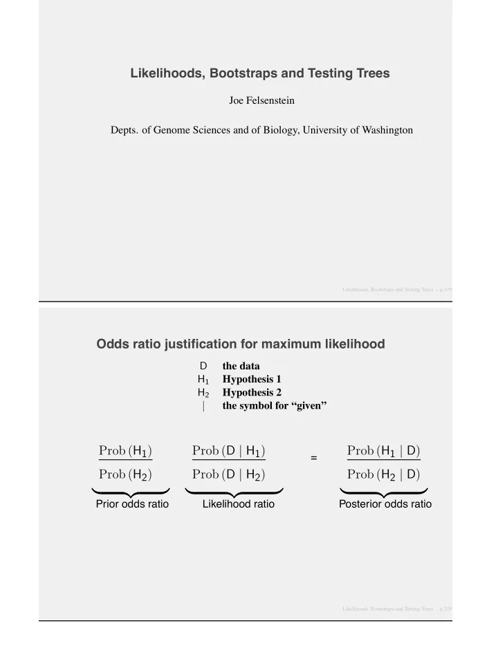
Prior odds ratio Likelihood ratio Posterior - PDF document

Likelihoods, Bootstraps and Testing Trees Joe Felsenstein Depts. of Genome Sciences and of Biology, University of Washington Likelihoods, Bootstraps and Testing Trees – p.1/59 Odds ratio justification for maximum likelihood the data D H 1 Hypothesis 1 Hypothesis 2 H 2 | the symbol for “given” Prob ( H 1 ) Prob ( D | H 1 ) Prob ( H 1 | D ) = Prob ( H 2 ) Prob ( D | H 2 ) Prob ( H 2 | D ) � �� � � �� � � �� � Prior odds ratio Likelihood ratio Posterior odds ratio Likelihoods, Bootstraps and Testing Trees – p.2/59

If a space probe finds no Little Green Men on Mars yes no priors no yes likelihoods no 1 yes 0 no yes no posteriors yes 1 × 1 / 3 4 × 1 / 3 4 4 1 1 = = 1 3 1 12 Likelihoods, Bootstraps and Testing Trees – p.3/59 The likelihood ratio term ultimately dominates If we see one Little Green Man, the likelihood calculation does the right thing: 4 × 2 / 3 ∞ 1 = 0 1 (put this way, this is OK but not mathematically kosher) If we send n space probes and keep seeing none, the likelihood ratio term is � 1 � n 3 It dominates the calculation, overwhelming the prior. Thus even if we don’t have a prior we can believe in, we may be interested in knowing which hypothesis the likelihood ratio is recommending ... Likelihoods, Bootstraps and Testing Trees – p.4/59

Likelihood in Simple Coin-Tossing Tossing a coin n times, with probability p of heads, the probability of outcome HHTHTTTTHTTH is pp ( 1 − p ) p ( 1 − p )( 1 − p )( 1 − p )( 1 − p ) p ( 1 − p )( 1 − p ) p which is L = p 5 ( 1 − p ) 6 Plotting L against p to find its maximum: Likelihood 0.0 0.2 0.4 0.6 0.8 1.0 0.454 p Likelihoods, Bootstraps and Testing Trees – p.5/59 Differentiating to find the maximum: Differentiating the expression for L with respect to p and equating the derivative to 0, the value of p that is at the peak is found (not surprisingly) to be p = 5 / 11 : � 5 � ∂ L 6 p 5 ( 1 − p ) 6 = 0 ∂ p = p − 1 − p 5 − 11 p = 0 5 ˆ p = 11 Likelihoods, Bootstraps and Testing Trees – p.6/59

A log-likelihood curve A Likelihood curve in one parameter Ln (Likelihood) length of a branch in the tree Likelihoods, Bootstraps and Testing Trees – p.7/59 Its maximum likelihood estimate A Likelihood curve in one parameter and the maximum likelihood estimate Ln (Likelihood) length of a branch in the tree maximum likelihood estimate (MLE) Likelihoods, Bootstraps and Testing Trees – p.8/59

The (approximate, asymptotic) confidence interval A Likelihood curve in one parameter and the maximum likelihood estimate and confidence interval derived from it 1/2 the value of a chi − square Ln (Likelihood) with 1 d.f. significant at 95% 95% confidence interval length of a branch in the tree maximum likelihood estimate (MLE) Likelihoods, Bootstraps and Testing Trees – p.9/59 Contours of a log-likelihood surface in two dimensions length of branch 2 MLE length of branch 1 Likelihoods, Bootstraps and Testing Trees – p.10/59

Log-likelihood-based confidence set for two variables shaded area is the joint confidence interval length of branch 2 height of this contour is less than at the peak by an amount equal to 1/2 the chi − square value with two degrees of freedom which is significant at 95% level length of branch 1 Likelihoods, Bootstraps and Testing Trees – p.11/59 Confidence interval for one variable length of branch 2 height of this contour is less than at the peak by an amount equal to 1/2 the chi − square value with one degree of freedom which is significant at 95% level length of branch 1 Likelihoods, Bootstraps and Testing Trees – p.12/59

Confidence interval for the other variable length of branch 2 height of this contour is less than at the peak by an amount equal to 1/2 the chi − square value with one degree of freedom which is significant at 95% level length of branch 1 Likelihoods, Bootstraps and Testing Trees – p.13/59 Calculating the likelihood of a tree If we have molecular sequences on a tree, the likelihood is the product over sites of the data D [ i ] for each site (if those evolve independently): sites � Prob ( D [ i ] | T ) = Prob ( D | T ) = L i = 1 With log-likelihoods, the product becomes a sum: sites � ln Prob ( D [ i ] | T ) ln L = ln Prob ( D | T ) = i = 1 Likelihoods, Bootstraps and Testing Trees – p.14/59

Calculating the likelihood for site i on a tree A C C C G t t 4 5 t1 t 2 t 3 y x t 6 t7 ti are z "branch lengths", (rate X time) t w 8 Sum over all possible states (bases) at interior nodes: � � � � L ( i ) = Prob ( w ) Prob ( x | w , t 7 ) x y z w × Prob ( A | x , t 1 ) Prob ( C | x , t 2 ) Prob ( z | w , t 8 ) × Prob ( C | z , t 3 ) Prob ( y | z , t 6 ) Prob ( C | y , t 4 ) Prob ( G | y , t 5 ) Likelihoods, Bootstraps and Testing Trees – p.15/59 Calculating the likelihood for site i on a tree We use the conditional likelihoods: L ( i ) j ( s ) These compute the probability of everything at site i at or above node j on the tree, given that node j is in state s . Thus it assumes something ( s ) that we don’t know in practice – so we compute these for all states s . At the tips we can define these quantities: if the observed state is (say) C , the vector of L ’s is ( 0 , 1 , 0 , 0 ) . If we observe an ambiguity, say R (purine), they are ( 1 , 0 , 1 , 0 ) , ( 1 / 2 , 0 , 1 / 2 , 0 ) not Likelihoods, Bootstraps and Testing Trees – p.16/59

The “pruning" algorithm: j k vj vk l � � � L ( i ) Prob ( s j | s , v j ) L ( i ) � ( s ) = j ( s j ) s j �� � Prob ( s k | s , v k ) L ( i ) × k ( s k ) s k (Felsenstein, 1973; 1981). Likelihoods, Bootstraps and Testing Trees – p.17/59 and at the bottom of the tree: � L ( i ) π s L ( i ) = 0 ( s ) 0 s (Felsenstein, 1973, 1981) and having gotten the likelihoods for each site: sites � L ( i ) L = 0 i = 1 Likelihoods, Bootstraps and Testing Trees – p.18/59

What does “tree space" (with branch lengths) look like? an example: three species with a clock trifurcation A B C not possible etc. t 1 t 1 t 2 OK t 2 when we consider all three possible topologies, the space looks like: t1 t1 t2 t2 Likelihoods, Bootstraps and Testing Trees – p.19/59 For one tree topology The space of trees varying all 2n − 3 branch lengths, each a nonegative number, defines an “orthant" (open corner) of a ( 2n − 3 ) -dimensional real space: B v 2 v w 3 wall a l l A v C 8 v v 1 7 v 9 v 4 D v 6 F f v 9 l o o r v 5 E Likelihoods, Bootstraps and Testing Trees – p.20/59

Through the looking-glass Shrinking one of the n − 1 interior branches to 0, we arrive at a trifurcation: B v 2 v 3 v A C 8 v v 1 7 v 9 v 4 D v 6 F v 5 E B v 2 v 3 A v C 8 v v 4 v 1 7 B B D v 2 v 2 v v 6 v v F 5 3 3 v C A v C 8 8 v v v 4 A v 1 5 v 9 7 E E v D v 1 v 9 7 v 6 F v v 4 5 v 6 F E D Here, as we pass “through the looking glass" we are also touch the space for two other tree topologies, and we could enter either. Likelihoods, Bootstraps and Testing Trees – p.21/59 The graph of all trees of 5 species C D D B A A B E E C C E D C B B D A A E A C B D E E B A B C A C D D E B D E B A A D B C B A C E D C A C E D E E C A B C A B D A B E D C D E A B D E C The Schoenberg graph (all 15 trees of size 5 connected by NNI’s) Likelihoods, Bootstraps and Testing Trees – p.22/59