Max. likelihood & Bayesian techniques are both likelihood-based. - PDF document

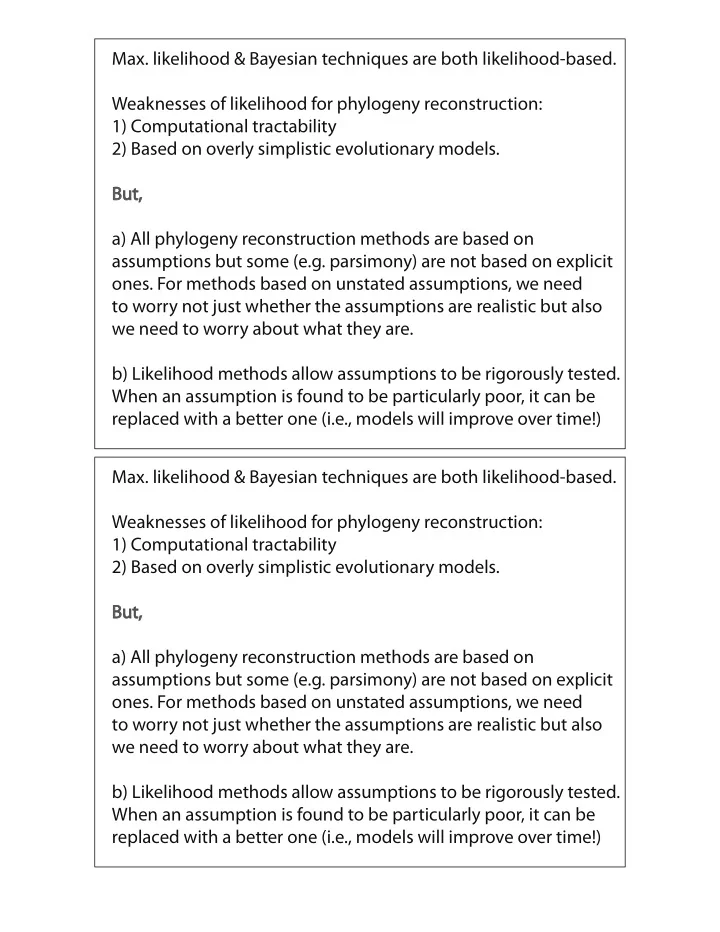
Max. likelihood & Bayesian techniques are both likelihood-based. Weaknesses of likelihood for phylogeny reconstruction: 1) Computational tractability 2) Based on overly simplistic evolutionary models. But, a) All phylogeny reconstruction methods are based on assumptions but some (e.g. parsimony) are not based on explicit ones. For methods based on unstated assumptions, we need to worry not just whether the assumptions are realistic but also we need to worry about what they are. b) Likelihood methods allow assumptions to be rigorously tested. When an assumption is found to be particularly poor, it can be replaced with a better one (i.e., models will improve over time!) Max. likelihood & Bayesian techniques are both likelihood-based. Weaknesses of likelihood for phylogeny reconstruction: 1) Computational tractability 2) Based on overly simplistic evolutionary models. But, a) All phylogeny reconstruction methods are based on assumptions but some (e.g. parsimony) are not based on explicit ones. For methods based on unstated assumptions, we need to worry not just whether the assumptions are realistic but also we need to worry about what they are. b) Likelihood methods allow assumptions to be rigorously tested. When an assumption is found to be particularly poor, it can be replaced with a better one (i.e., models will improve over time!)

Strengths of likelihood methods: 1. Explicit Assumptions – we know what we’re assuming. 2. Use all information in a data set. Distance methods, for example, do not. This is part of the explanation for success of likelihood methods in simulations – they tend to yield estimates that are closer to the truth than other methods. 3. Likelihood approaches are consistent. Estimates get better as amount of data increases. (Caveat: violation of model assumptions may cause loss of consistency property) 4. Because likelihood applied to so many statistical situations in addition to phylogenetics, powerful theory & tools for performing likelihood analyses have developed. This theory and these tools (e.g., tools for hypothesis testing) can be applied to phylogenetics. 5. Likelihood lets you know how good estimate is, in addition to what estimate is. Mechanistic versus Phenomenological Models of Sequence Evolution see Ph.D. thesis by Nicolas Rodrigue (”Phylogenetic structural modeling of molecular evolution” , 2008, University of Montreal) (see also Rodrigue & Philippe. 2010. Trends in Genetics 26:248-252)

One good idea for more realistic models ... TUFFLEY, C., and M. A. STEEL. 1998. Modeling the covarion hypothesis of nucleotide substitution. Math. Biosci. 147:63–91. From Galtier. 2001. Mol. Biol. Evol. 18(5):866-873.

Tuffley/Steel -type model Slow Fast A C G T A C G T A - r r r f 0 0 0 S C r - r r 0 f 0 0 l o G r r - r 0 0 f 0 w T r r r - 0 0 0 f A s 0 0 0 - q q q F C 0 s 0 0 q - q q a s G 0 0 s 0 q q - q t T 0 0 0 s q q q - Substitution Rates: q>r Switching rates: f (slow to fast), s (fast to slow) Dayhoff model of protein evolution (see Dayhoff et al. 1972; Dayhoff et al. 1978) operates at the level of the 20 amino acid types. π is the probability of amino acid type i i α is the instantaneous rate of replacement from amino acid i ij to amino acid j Dayhoff model is most general time-reversible 20-state model of amino acid replacement. This means π α = π α for all i and j. i ij ji j

It is important to separate the Dayhoff model of protein evolution from: 1. The procedure used by Dayhoff and collaborators to estimate the α AND ij 2. The data set upon which the α estimates were based. ij Dayhoff and collaborators exploited the fact that the probability of replacements from amino acid type i to type j (i not equal to j) is approximately linear in time for small amounts of time. In other words, the probability of a replacement from amino acid type i to a different type j is approximately α t if t represents some ij small amount of time. Subsequent studies (e.g., Jones et al. 1992) adopted the Dayhoff model but employed different data sets and parameter estimation procedures.

�������������������������������������������������� ������������������������������������������������ ����������������������������������������������� ��������������������������������������������� ����������������������������������������������������� ������������������������������������������������ ����������������������������������������������������� ����������� ��������������� �������������������������������������� ����������������������������������������������������� ������������ Ni c o l as Larti ll ot and H erv é Phi l ippe. 2004. A Bayesian Mixture Mode l for A c ross-Site H eterogeneities in the Amino-A c id Rep l a c ement Pro c ess. Mo l . Bio l . Evo l . 2 1 (6): 1 0 9 5- 11 0 9 . 2004 Diri c h l et Pro c ess Priors (”Chinese restaurant pro c ess” , not same as Diri c h l et distribution): Usefu l to spe c ify prior distribution for situations when number of c ategories is unknown and where prior probabi l ity of ea c h possib l e c ategory needs determination. Additiona l app l i c ations in Evo l ution I n cl ude: Chara c teri z ation of popu l ation stru c ture H ue l senbe c k and Ando l fatto. 200 7 . Geneti c s. 17 5: 17 8 7 - 1 802. V ariation in nonsyn. and synonymous rates among sites H ue l senbe c k et a l . 2006. PNAS 1 03( 1 6): 6263-6268. V ariation in evo l utionary rate a c ross a phy l ogeny H eath et a l . 20 1 2. Mo l . Bio l . Evo l . 2 9 (3): 9 3 9 - 9 55.

Codon Models: Evolution occurs at the DNA level rather than at the amino acid level. It makes sense to frame a model of protein evolution in terms of codons rather than amino acid types (Schoniger et al. 1990; Goldman and Yang 1994; Muse and Gaut 1994). Codon-based models are typically framed in terms of 61 codon- states rather than 64 codon-states because the common genetic codes have three stop codons, and the possibility that a stop codon may appear or disappear from a sequence is not allowed. One simplification that is often adopted holds that changes from one codon to another are only possible when the two codons differ at exactly one of the three codon positions. The instantaneous rates of other changes between codons are set to 0. Typical parameterization of a codon model when physicochemical differences between amino acids are ignored... Instantaneous rate α i,j from codon i to codon j is set to 0 if i and j differ at more than one nucleotide or if j encodes a premature stop codon. For cases where i and j differ by exactly one nucleotide, rate matrix entries are: ⎧ for a synonymous transversion uπ j ⎪ ⎪ ⎪ ⎪ ⎪ ⎪ for a synonymous transition ⎪ uπ j κ ⎪ ⎪ ⎪ α i,j = ⎨ for a nonsynonymous transversion uπ j ω ⎪ ⎪ ⎪ ⎪ ⎪ ⎪ ⎪ uπ j κω for a nonsynonymous transition ⎪ ⎪ ⎪ ⎩ u , π j , and κ reflect mutation rates ω > 1 means positive diversifying selection (i.e., nonsyn. rates higher than they would be if changes were synonymous) Other kinds of positive selection exist (e.g., positive directional se- lection)