Maximum-likelihood and Bayesian parameter estimation Andrea - PowerPoint PPT Presentation

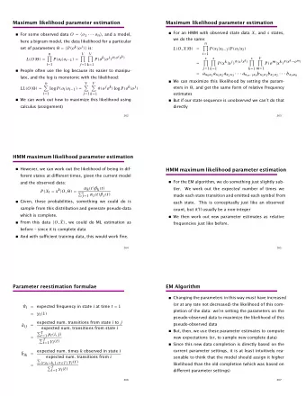
Maximum-likelihood and Bayesian parameter estimation Andrea Passerini passerini@disi.unitn.it Machine Learning Maximum-likelihood and Bayesian parameter estimation

Parameter estimation Setting Data are sampled from a probability distribution p ( x , y ) The form of the probability distribution p is known but its parameters are unknown There is a training set D = { ( x 1 , y 1 ) , . . . , ( x m , y m ) } of examples sampled i.i.d. according to p ( x , y ) Task Estimate the unknown parameters of p from training data D . Note: i.i.d. sampling independent : each example is sampled independently from the others identically distributed: all examples are sampled from the same distribution Maximum-likelihood and Bayesian parameter estimation

Parameter estimation Multiclass classification setting The training set can be divided into D 1 , . . . , D c subsets, one for each class ( D i = { x 1 , . . . , x n } contains i.i.d examples for target class y i ) For any new example x (not in training set), we compute the posterior probability of the class given the example and the full training set D : P ( y i | x , D ) = p ( x | y i , D ) p ( y i |D ) p ( x |D ) Note same as Bayesian decision theory (compute posterior probability of class given example) except that parameters of distributions are unknown a training set D is provided instead Maximum-likelihood and Bayesian parameter estimation

Parameter estimation Multiclass classification setting: simplifications P ( y i | x , D ) = p ( x | y i , D i ) p ( y i |D ) p ( x |D ) we assume x is independent of D j ( j � = i ) given y i and D i without additional knowledge, p ( y i |D ) can be computed as the fraction of examples with that class in the dataset the normalizing factor p ( x |D ) can be computed marginalizing p ( x | y i , D i ) p ( y i |D ) over possible classes Note We must estimate class-dependent parameters θ i for: p ( x | y i , D i ) Maximum-likelihood and Bayesian parameter estimation

Maximum Likelihood vs Bayesian estimation Maxiumum likelihood/Maximum a-posteriori estimation Assumes parameters θ i have fixed but unknown values Values are computed as those maximizing the probability of the observed examples D i (the training set for the class) Obtained values are used to compute probability for new examples: p ( x | y i , D i ) ≈ p ( x | θ i ) Maximum-likelihood and Bayesian parameter estimation

Maximum Likelihood vs Bayesian estimation Bayesian estimation Assumes parameters θ i are random variables with some known prior distribution Observing examples turns prior distribution over parameters into a posterior distribution Predictions for new examples are obtained integrating over all possible values for the parameters: � p ( x | y i , D i ) = p ( x , θ i | y i , D i ) d θ i θ i Maximum-likelihood and Bayesian parameter estimation

Maxiumum likelihood/Maximum a-posteriori estimation Maximum a-posteriori estimation θ ∗ i = argmax θ i p ( θ i |D i , y i ) = argmax θ i p ( D i , y i | θ i ) p ( θ i ) Assumes a prior distribution for the parameters p ( θ i ) is available Maximum likelihood estimation (most common) θ ∗ i = argmax θ i p ( D i , y i | θ i ) maximizes the likelihood of the parameters with respect to the training samples no assumption about prior distributions for parameters Note Each class y i is treated independently: replace y i , D i → D for simplicity Maximum-likelihood and Bayesian parameter estimation

Maximum-likelihood (ML) estimation Setting (again) A training data D = { x 1 , . . . , x n } of i.i.d. examples for the target class y is available We assume the parameter vector θ has a fixed but unknown value We estimate such value maximizing its likelihood with respect to the training data: n � θ ∗ = argmax θ p ( D| θ ) = argmax θ p ( x j | θ ) j = 1 The joint probability over D decomposes into a product as examples are i.i.d (thus independent of each other given the distribution) Maximum-likelihood and Bayesian parameter estimation

Maximum-likelihood estimation Maximizing log-likelihood It is usually simpler to maximize the logarithm of the likelihood (monotonic): n � θ ∗ = argmax θ ln p ( D| θ ) = argmax θ ln p ( x j | θ ) j = 1 Necessary conditions for the maximum can be obtained zeroing the gradient wrt to θ : n � ∇ θ ln p ( x j | θ ) = 0 j = 1 Points zeroing the gradient can be local or global maxima depending on the form of the distribution Maximum-likelihood and Bayesian parameter estimation

Maximum-likelihood estimation Univariate Gaussian case: unknown µ and σ 2 the log-likelihood is: n − 1 2 σ 2 ( x j − µ ) 2 − 1 � 2 ln 2 πσ 2 L = j = 1 The gradient wrt µ is: n n ∂ L − 1 1 � � ∂µ = 2 2 σ 2 ( x j − µ )( − 1 ) = σ 2 ( x j − µ ) j = 1 j = 1 Maximum-likelihood and Bayesian parameter estimation

Maximum-likelihood estimation Univariate Gaussian case: unknown µ and σ 2 Setting the gradient to zero gives mean: n n 1 � � σ 2 ( x j − µ ) = 0 = ( x j − µ ) j = 1 j = 1 n n � � x j = µ j = 1 j = 1 n � x j = n µ j = 1 n µ = 1 � x j n j = 1 Maximum-likelihood and Bayesian parameter estimation

Maximum-likelihood estimation Univariate Gaussian case: unknown µ and σ 2 the log-likelihood is: n − 1 2 σ 2 ( x j − µ ) 2 − 1 � 2 ln 2 πσ 2 L = j = 1 The gradient wrt σ 2 is: n ∂ L − ( x j − µ ) 2 ∂ 2 σ 2 − 1 1 1 � ∂σ 2 = 2 πσ 2 2 π ∂σ 2 2 j = 1 n − ( x j − µ ) 2 1 2 ( − 1 ) 1 1 � = σ 4 − 2 σ 2 j = 1 Maximum-likelihood and Bayesian parameter estimation

Maximum-likelihood estimation Univariate Gaussian case: unknown µ and σ 2 Setting the gradient to zero gives variance: n n ( x j − µ ) 2 1 � � 2 σ 2 = 2 σ 4 j = 1 j = 1 n n � � σ 2 = ( x j − µ ) 2 j = 1 j = 1 n σ 2 = 1 � ( x j − µ ) 2 n j = 1 Maximum-likelihood and Bayesian parameter estimation

Maximum-likelihood estimation Multivariate Gaussian case: unknown µ and Σ the log-likelihood is: n − 1 2 ( x j − µ ) t Σ − 1 ( x j − µ ) − 1 � 2 ln ( 2 π ) d | Σ | j = 1 The maximum-likelihood estimates are: n µ = 1 � x j n j = 1 and: n Σ = 1 � ( x j − µ )( x j − µ ) t n j = 1 Maximum-likelihood and Bayesian parameter estimation

Maximum-likelihood estimation general Gaussian case: Maximum likelihood estimates for Gaussian parameters are simply their empirical estimates over the samples: Gaussian mean is the sample mean Gaussian covariance matrix is the mean of the sample covariances Maximum-likelihood and Bayesian parameter estimation

Bayesian estimation setting (again) Assumes parameters θ i are random variables with some known prior distribution Predictions for new examples are obtained integrating over all possible values for the parameters: � p ( x | y i , D i ) = p ( x , θ i | y i , D i ) d θ i θ i probability of x given each class y i is independent of the other classes y j , for simplicity we can again write: � p ( x | y i , D i ) → p ( x |D ) = p ( x , θ |D ) d θ θ where D is a dataset for a certain class y and θ the parameters of the distribution Maximum-likelihood and Bayesian parameter estimation

Bayesian estimation setting � � p ( x |D ) = p ( x , θ |D ) d θ = p ( x | θ ) p ( θ |D ) d θ θ p ( x | θ ) can be easily computed (we have both form and parameters of distribution, e.g. Gaussian) need to estimate the parameter posterior density given the training set: p ( θ |D ) = p ( D| θ ) p ( θ ) p ( D ) Maximum-likelihood and Bayesian parameter estimation

Bayesian estimation denominator p ( θ |D ) = p ( D| θ ) p ( θ ) p ( D ) p ( D ) is a constant independent of θ (i.e. it will no influence final Bayesian decision) if final probability (not only decision) is needed we can compute: � p ( D ) = p ( D| θ ) p ( θ ) d θ θ Maximum-likelihood and Bayesian parameter estimation

Bayesian estimation Univariate normal case: unknown µ , known σ 2 Examples are drawn from: p ( x | µ ) ∼ N ( µ, σ 2 ) The Gaussian mean prior distribution is itself normal: p ( µ ) ∼ N ( µ 0 , σ 2 0 ) The Gaussian mean posterior given the dataset is computed as: n p ( µ |D ) = p ( D| µ ) p ( µ ) � = α p ( x j | µ ) p ( µ ) p ( D ) j = 1 where α = 1 / p ( D ) is independent of µ Maximum-likelihood and Bayesian parameter estimation

Univariate normal case: unknown µ , known σ 2 a posteriori parameter density p ( x j | µ ) p ( µ ) � �� � � �� � � � 2 � � � 2 � n � x j − µ � µ − µ 0 1 − 1 1 − 1 � √ √ p ( µ |D ) = α exp exp σ σ 0 2 2 2 πσ 2 πσ 0 j = 1     n � µ − x j � 2 � µ − µ 0 � 2  − 1 � = α ′ exp +    σ σ 0 2 j = 1       � n n �  − 1 σ 2 + 1  1 x j + µ 0 � = α ′′ exp µ 2 − 2  µ    2 σ 2 σ 2 σ 2 0 0 j = 1 Normal distribution � � 2 � � µ − µ n 1 − 1 p ( µ |D ) = √ exp 2 σ n 2 πσ n Maximum-likelihood and Bayesian parameter estimation