4CSLL5 Parameter Estimation (Supervised and Unsupervised) - PowerPoint PPT Presentation

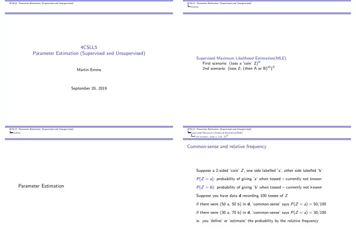
4CSLL5 Parameter Estimation (Supervised and Unsupervised) 4CSLL5 Parameter Estimation (Supervised and Unsupervised) Outline 4CSLL5 Parameter Estimation (Supervised and Unsupervised) Supervised Maximum Likelihood Estimation(MLE) First scenario: (toss a ’coin’ Z) D 2nd scenario: (toss Z; (then A or B) 10 ) D Martin Emms September 20, 2019 4CSLL5 Parameter Estimation (Supervised and Unsupervised) 4CSLL5 Parameter Estimation (Supervised and Unsupervised) Outline Supervised Maximum Likelihood Estimation(MLE) First scenario: (toss a ’coin’ Z) D Common-sense and relative frequency Suppose a 2-sided ’coin’ Z , one side labelled ’a’, other side labelled ’b’ P ( Z = a ): probability of giving ’a’ when tossed – currently not known Parameter Estimation P ( Z = b ): probability of giving ’b’ when tossed – currently not known Suppose you have data d recording 100 tosses of Z if there were (50 a, 50 b) in d , ’common-sense’ says P ( Z = a ) = 50 / 100 if there were (30 a, 70 b) in d , ’common-sense’ says P ( Z = a ) = 30 / 100 ie. you ’define’ or ’estimate’ the probability by the relative frequency

4CSLL5 Parameter Estimation (Supervised and Unsupervised) 4CSLL5 Parameter Estimation (Supervised and Unsupervised) Supervised Maximum Likelihood Estimation(MLE) Supervised Maximum Likelihood Estimation(MLE) First scenario: (toss a ’coin’ Z) D First scenario: (toss a ’coin’ Z) D Data likelihood p ( d ) for 50 a, 50 b assuming the tosses of Z are all independent, can work out the probability of X 1.2e−21 the observed data d if Z ’s probabilities had particular values. let θ a and θ b stand for P ( Z = a ) and P ( Z = b ) as θ a is varied, data prob p ( d ) varies 8.0e−22 let #( a ) be the number of ’a’ outcomes in the sequence d let #( b ) be the number of ’b’ outcomes in the sequence d max occurs at θ a = 0 . 5 4.0e−22 the probability of d , assuming the probability settings θ a and θ b is 50 which is 50 + 50 p ( d ) = θ #( a ) × θ #( b ) (1) a b 0.0e+00 different settings of θ a and θ b will give different values for p ( d ) 0.0 0.2 0.4 0.6 0.8 1.0 following slides investigate this empirically 4CSLL5 Parameter Estimation (Supervised and Unsupervised) 4CSLL5 Parameter Estimation (Supervised and Unsupervised) Supervised Maximum Likelihood Estimation(MLE) Supervised Maximum Likelihood Estimation(MLE) First scenario: (toss a ’coin’ Z) D First scenario: (toss a ’coin’ Z) D p ( d ) for 30 a, 70 b p ( d ) for 70 a, 30 b 4e−19 4e−19 X X 3e−19 3e−19 as θ a is varied, data prob p ( d ; θ a , θ b ) as θ a is varied, data prob p ( d ; θ a , θ b ) varies varies 2e−19 2e−19 max occurs at θ a = 0 . 3 max occurs at θ a = 0 . 7 1e−19 30 1e−19 70 which is which is 30 + 70 70 + 30 0e+00 0e+00 0.0 0.2 0.4 0.6 0.8 1.0 0.0 0.2 0.4 0.6 0.8 1.0

4CSLL5 Parameter Estimation (Supervised and Unsupervised) 4CSLL5 Parameter Estimation (Supervised and Unsupervised) Supervised Maximum Likelihood Estimation(MLE) Supervised Maximum Likelihood Estimation(MLE) First scenario: (toss a ’coin’ Z) D First scenario: (toss a ’coin’ Z) D ◮ in each case, it looks like the max of the data probability occured at the on reflection, if you have to set parameters given data, it makes a lot of sense value given by the relative frequency to set the parameters to whatever values make the data as likely as possible ◮ this suggests that in these cases, formula for p ( d ; θ a , θ b ) is (1), repeated below Max. Likelihood Estimator if you wanted to find θ a (and θ b ) that maximise the data probability, that is you p ( d ; θ a , θ b ) = θ #( a ) × θ #( b ) a b want and because θ b = 1 − θ a can really write this in terms of just parameter θ a arg max p ( d ; θ a , θ b ) θ a ,θ b p ( d ; θ a ) = θ #( a ) × (1 − θ a ) #( b ) a then the relative frequencies would give the answer, that is Looking at some pics suggested a formula for the value of θ a that maximises #( a ) #( b ) this. Can we actually derive this formula? θ a = θ b = #( a ) + #( b ) #( a ) + #( b ) Yes ⇒ take the log of this – the log-likelihood and use calculus to maximize that w.r.t. θ a – this turns out to be (relatively) easy ◮ technically expressed as: the relative frequency is a maximum likelihood estimator of the parameters 4CSLL5 Parameter Estimation (Supervised and Unsupervised) 4CSLL5 Parameter Estimation (Supervised and Unsupervised) Supervised Maximum Likelihood Estimation(MLE) Supervised Maximum Likelihood Estimation(MLE) First scenario: (toss a ’coin’ Z) D 2nd scenario: (toss Z; (then A or B)10) D a more complex scenario suppose D repetitions of Define L ( θ a ) as log ( P ( d ; θ a )). Then you get toss disc Z , to choose one of two coins A or B then toss chosen coin 10 times L ( θ a ) = #( a ) log θ a + #( b ) log(1 − θ a ) Suppose 9 repetitions gave d Z X : tosses of chosen coin H counts need to take derivative wrt to θ a and set to 0, which is 1 A H H H H H H H H T T (8H) 2 B T T H T T T H T T T (2H) dL ( θ a ) #( a ) − #( b ) #( a ) + #( b ) = #( a ) #( a ) 3 A H T H H T H H H H T (7H) = 1 − θ a = 0 = θ a = ⇒ 4 A H T H H H T H H H H (8H) d θ a θ a 100 5 B T T T T T T H T T T (1H) 6 A H H T H H H H H H H (9H) so in this scenario of 100 tosses of Z , we have proven that the relative 7 A T H H T H H H H H T (7H) frequency is always going to the maximum likelihood estimator 8 A H H H H H H T H H H (9H) now want to consider slightly more complex scenario 9 B H H T T T T T H T T (3H) Let θ a be Z ’s probability of giving A Let θ h | a be A ’s probability of giving H Let θ h | b be B ’s probability of giving H

4CSLL5 Parameter Estimation (Supervised and Unsupervised) 4CSLL5 Parameter Estimation (Supervised and Unsupervised) Supervised Maximum Likelihood Estimation(MLE) Supervised Maximum Likelihood Estimation(MLE) 2nd scenario: (toss Z; (then A or B)10) D 2nd scenario: (toss Z; (then A or B)10) D ’common sense’ calculation of θ a , θ h | a and θ h | b to make the comparision with the hidden variable version which will come up for θ a , need ( count of Z = A cases )/( count of all Z cases ), ie. later, its worth noting that we can formulate all the restricted sums � d : Z = A (Φ( d )) with unrestricted sums if we put a so-called Kronecker-delta � d : Z = A 1 = 6 indicator function inside the sum � d ( δ ( d , A )Φ( d )) where δ ( d , A ) = 1 if datum est ( θ a ) = 9 = 0 . 66 (2) D d had Z = A , and is 0 otherwise. � d δ ( d , A ) for θ h | a , need est ( θ a ) = (5) ( count of H when A chosen )/( count of all tosses when A chosen ), ie. D � d : Z = A #( d , h ) = 48 60 = 4 est ( θ h | a ) = 5 = 0 . 8 (3) � d δ ( d , A )#( d , h ) � d : Z = A 10 est ( θ h | a ) = (6) � d δ ( d , A )10 for θ h | b , need ( count of H when B chosen )/( count of all tosses when B chosen ), ie. � d δ ( d , B )#( d , h ) est ( θ h | b ) = (7) � d : Z = B #( d , h ) = 6 30 = 1 � d δ ( d , B )10 est ( θ h | b ) = 5 = 0 . 2 (4) � d : Z = B 10 4CSLL5 Parameter Estimation (Supervised and Unsupervised) Supervised Maximum Likelihood Estimation(MLE) 2nd scenario: (toss Z; (then A or B)10) D � [ log θ a + #( d , h ) log θ h | a + #( d , t ) log θ t | a ]+ d : Z = a it turns out that in this scenario also, the ’common-sense’, relative-frequency � [ log θ b + #( d , h ) log θ h | b + #( d , t ) log θ t | b ] answers are also maximum likelihood estimators ie. values which maximise the d : Z = b probability of the data, and again it is (relatively) easy to show this by taking logs and using calculus. L ( θ a , θ h | a , θ h | b ) – repeated above – can be split into 3 separate terms, L ( θ a ) + L ( θ h | a ) + L ( θ h | b ) concerning Z, A and B the formula for p ( d ; θ a , θ b , θ h | a , θ t | a , θ h | b , θ t | b ) � [ θ a θ #( d , h ) θ #( d , t ) � [ θ b θ #( d , h ) θ #( d , t ) p ( d ) = ] ] � � L ( θ a ) = [ 1] log θ a + [ 1] log (1 − θ a ) (8) h | a t | a h | b t | b d : Z = a d : Z = b d : Z = a d : Z = b � � L ( θ h | a ) = [ #( d , h )] log θ h | a + [ #( d , t )] log (1 − θ h | a ) (9) and its log comes out as d : Z = a d : Z = a � � L ( θ h | b ) = [ #( d , h )] log θ h | b + [ #( d , t )] log (1 − θ h | b ) (10) � [ log θ a + #( d , h ) log θ h | a + #( d , t ) log θ t | a ]+ d : Z = b d : Z = b d : Z = a and this means that when you take the derivatives of L ( θ a , θ h | a , θ h | b ) wrt. θ a , � [ log θ b + #( d , h ) log θ h | b + #( d , t ) log θ t | b ] θ h | a and θ h | b in each case you can just look at one of the above terms. They are d : Z = b all really of the same form being N ( log ( p )) + M ( log (1 − p )), the same form as N seen in the first simple scenario, and it has maximum value at p = call this L ( θ a , θ h | a , θ h | b ) N + M

4CSLL5 Parameter Estimation (Supervised and Unsupervised) Supervised Maximum Likelihood Estimation(MLE) 2nd scenario: (toss Z; (then A or B)10) D hence � d : Z = a 1 ∂ L ( θ a ) = 0 = ⇒ θ a = ∂θ a � d : Z = a 1 + � d : Z = b 1 ∂ L ( θ h | a ) � d : Z = a #( d , h ) = 0 = ⇒ θ h | a = ∂θ h | a � d : Z = a #( d , h ) + � d : Z = a #( d , t ) ∂ L ( θ h | b ) � d : Z = b #( d , h ) = 0 = ⇒ θ h | b = ∂θ h | b � d : Z = b #( d , h ) + � d : Z = b #( d , t ) finally the denominators of these turn into D , � d : Z = a 10 and � d : Z = b 10 respectively and so are exactly the ’common sense’ formulae we started with in (2), (3), (4)