Recap: N -gram models ANLP Lecture 6 We can model sentence probs by - PowerPoint PPT Presentation
Recap: N -gram models ANLP Lecture 6 We can model sentence probs by conditioning each word on N 1 N-gram models and smoothing previous words. For example, a bigram model: Sharon Goldwater n (some slides from Philipp Koehn) P (
Recap: N -gram models ANLP Lecture 6 • We can model sentence probs by conditioning each word on N − 1 N-gram models and smoothing previous words. • For example, a bigram model: Sharon Goldwater n (some slides from Philipp Koehn) � P ( � w ) = P ( w i | w i − 1 ) 26 September 2019 i =1 • Or trigram model: n � P ( � w ) = P ( w i | w i − 2 , w i − 1 ) i =1 Sharon Goldwater ANLP Lecture 6 26 September 2019 Sharon Goldwater ANLP Lecture 6 1 MLE estimates for N -grams MLE estimates for N -grams • To estimate each word prob, we could use MLE... • To estimate each word prob, we could use MLE... C ( w 1 , w 2 ) C ( w 1 , w 2 ) P ML ( w 2 | w 1 ) = P ML ( w 2 | w 1 ) = C ( w 1 ) C ( w 1 ) • But what happens when I compute P (consuming | commence) ? • But what happens when I compute P (consuming | commence) ? – Assume we have seen commence in our corpus – Assume we have seen commence in our corpus – But we have never seen commence consuming – But we have never seen commence consuming • Any sentence with commence consuming gets probability 0 The guests shall commence consuming supper Green inked commence consuming garden the Sharon Goldwater ANLP Lecture 6 2 Sharon Goldwater ANLP Lecture 6 3
The problem with MLE Today’s lecture: • MLE estimates probabilities that make the observed data • How does add-alpha smoothing work, and what are its effects? maximally probable • What are some more sophisticated smoothing methods, and what • by assuming anything unseen cannot happen (and also assigning information do they use that simpler methods don’t? too much probability to low-frequency observed events). • What are training, development, and test sets used for? • It over-fits the training data. • What are the trade-offs between higher order and lower order • We tried to avoid zero-probability sentences by modelling with n-grams? smaller chunks ( n -grams), but even these will sometimes have zero prob under MLE. • What is a word embedding and how can it help in language modelling? Today: smoothing methods, which reassign probability mass from observed to unobserved events, to avoid overfitting/zero probs. Sharon Goldwater ANLP Lecture 6 4 Sharon Goldwater ANLP Lecture 6 5 Add-One Smoothing Add-One Smoothing • For all possible bigrams, add one more count. • For all possible bigrams, add one more count. P ML ( w i | w i − 1 ) = C ( w i − 1 , w i ) P ML ( w i | w i − 1 ) = C ( w i − 1 , w i ) C ( w i − 1 ) C ( w i − 1 ) P +1 ( w i | w i − 1 ) = C ( w i − 1 , w i ) + 1 P +1 ( w i | w i − 1 ) = C ( w i − 1 , w i ) + 1 ⇒ ? ⇒ ? C ( w i − 1 ) C ( w i − 1 ) • NO! Sum over possible w i (in vocabulary V ) must equal 1: � P ( w i | w i − 1 ) = 1 w i ∈ V • True for P ML but we increased the numerator; must change denominator too. Sharon Goldwater ANLP Lecture 6 6 Sharon Goldwater ANLP Lecture 6 7
Add-One Smoothing: normalization Add-One Smoothing: effects C ( w i − 1 , w i ) + 1 • We want: • Add-one smoothing: � = 1 C ( w i − 1 ) + x w i ∈ V P +1 ( w i | w i − 1 ) = C ( w i − 1 , w i ) + 1 C ( w i − 1 ) + v • Solve for x : � ( C ( w i − 1 , w i ) + 1) = C ( w i − 1 ) + x w i ∈ V • Large vobulary size means v is often much larger than C ( w i − 1 ) , � � C ( w i − 1 , w i ) + 1 = C ( w i − 1 ) + x overpowers actual counts. w i ∈ V w i ∈ V C ( w i − 1 ) + v = C ( w i − 1 ) + x • Example: in Europarl, v = 86 , 700 word types (30m tokens, max C ( w i − 1 ) = 2m). • So, P +1 ( w i | w i − 1 ) = C ( w i − 1 ,w i )+1 where v = vocabulary size. C ( w i − 1 )+ v Sharon Goldwater ANLP Lecture 6 8 Sharon Goldwater ANLP Lecture 6 9 Add-One Smoothing: effects The problem with Add-One smoothing P +1 ( w i | w i − 1 ) = C ( w i − 1 , w i ) + 1 • All smoothing methods “steal from the rich to give to the poor” C ( w i − 1 ) + v Using v = 86 , 700 compute some example probabilities: • Add-one smoothing steals way too much • ML estimates for frequent events are quite accurate, don’t want C ( w i − 1 ) = 10 , 000 C ( w i − 1 ) = 100 smoothing to change these much. C ( w i − 1 , w i ) P ML = P +1 ≈ C ( w i − 1 , w i ) P ML = P +1 ≈ 100 1/100 1/970 100 1 1/870 10 1/1k 1/10k 10 1/10 1/9k 1 1/10k 1/48k 1 1/100 1/43k 0 0 1/97k 0 0 1/87k Sharon Goldwater ANLP Lecture 6 10 Sharon Goldwater ANLP Lecture 6 11
Add- α Smoothing Optimizing α • Divide corpus into training set (80-90%), held-out (or • Add α < 1 to each count development or validation ) set (5-10%), and test set (5-10%) P + α ( w i | w i − 1 ) = C ( w i − 1 , w i ) + α • Train model (estimate probabilities) on training set with different C ( w i − 1 ) + αv values of α • Choose the value of α that minimizes perplexity on dev set • Simplifying notation: c is n-gram count, n is history count P + α = c + α • Report final results on test set n + αv • What is a good value for α ? Sharon Goldwater ANLP Lecture 6 12 Sharon Goldwater ANLP Lecture 6 13 A general methodology Is add- α sufficient? • Training/dev/test split is used across machine learning • Even if we optimize α , add- α smoothing makes pretty bad predictions for word sequences. • Development set used for evaluating different models, debugging, optimizing parameters (like α ) • Some cleverer methods such as Good-Turing improve on this by discounting less from very frequent items. But there’s still a • Test set simulates deployment; only used once final model and problem... parameters are chosen. (Ideally: once per paper) • Avoids overfitting to the training set and even to the test set Sharon Goldwater ANLP Lecture 6 14 Sharon Goldwater ANLP Lecture 6 15
Remaining problem Remaining problem • In given corpus, suppose we never observe • Previous smoothing methods assign equal probability to all unseen events. – Scottish beer drinkers – Scottish beer eaters • Better: use information from lower order N -grams (shorter histories). • If we build a trigram model smoothed with Add- α or G-T, which example has higher probability? – beer drinkers – beer eaters • Two ways: interpolation and backoff . Sharon Goldwater ANLP Lecture 6 16 Sharon Goldwater ANLP Lecture 6 17 Interpolation Interpolation • Higher and lower order N -gram models have different strengths • Note that λ i s must sum to 1: and weaknesses – high-order N -grams are sensitive to more context, but have � 1 = P I ( w 3 | w 1 , w 2 ) sparse counts w 3 – low-order N -grams consider only very limited context, but have � = [ λ 1 P 1 ( w 3 ) + λ 2 P 2 ( w 3 | w 2 ) + λ 3 P 3 ( w 3 | w 1 , w 2 )] robust counts w 3 � � � • So, combine them: = λ 1 P 1 ( w 3 ) + λ 2 P 2 ( w 3 | w 2 ) + λ 3 P 3 ( w 3 | w 1 , w 2 ) P I ( w 3 | w 1 , w 2 ) = λ 1 P 1 ( w 3 ) P 1 (drinkers) w 3 w 3 w 3 = λ 1 + λ 2 + λ 3 + λ 2 P 2 ( w 3 | w 2 ) P 2 (drinkers | beer) + λ 3 P 3 ( w 3 | w 1 , w 2 ) P 3 (drinkers | Scottish , beer) Sharon Goldwater ANLP Lecture 6 18 Sharon Goldwater ANLP Lecture 6 19
Fitting the interpolation parameters Back-Off • In general, any weighted combination of distributions is called a • Trust the highest order language model that contains N -gram, mixture model . otherwise “back off” to a lower order model. • So λ i s are interpolation parameters or mixture weights . • Basic idea: – discount the probabilities slightly in higher order model • The values of the λ i s are chosen to optimize perplexity on a – spread the extra mass between lower order N -grams held-out data set. • But maths gets complicated to make probabilities sum to 1. Sharon Goldwater ANLP Lecture 6 20 Sharon Goldwater ANLP Lecture 6 21 Back-Off Equation Do our smoothing methods work here? Example from MacKay and Bauman Peto (1994): P BO ( w i | w i − N +1 , ..., w i − 1 ) = Imagine, you see, that the language, you see, has, you see, P ∗ ( w i | w i − N +1 , ..., w i − 1 ) a frequently occurring couplet, ‘you see’, you see, in which if count ( w i − N +1 , ..., w i ) > 0 the second word of the couplet, ‘see’, follows the first word, = ‘you’, with very high probability, you see. Then the marginal α ( w i − N +1 , ..., w i − 1 ) P BO ( w i | w i − N +2 , ..., w i − 1 ) statistics, you see, are going to become hugely dominated, else you see, by the words ‘you’ and ‘see’, with equal frequency, • Requires you see. – adjusted prediction model P ∗ ( w i | w i − N +1 , ..., w i − 1 ) – backoff weights α ( w 1 , ..., w N − 1 ) • P ( see ) and P ( you ) both high, but see nearly always follows you . • See textbook for details/explanation. • So P ( see | novel ) should be much lower than P ( you | novel ) . Sharon Goldwater ANLP Lecture 6 22 Sharon Goldwater ANLP Lecture 6 23
Recommend
More recommend
Explore More Topics
Stay informed with curated content and fresh updates.
