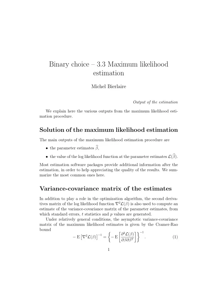
Binary choice 3.3 Maximum likelihood estimation Michel Bierlaire - PDF document

Binary choice – 3.3 Maximum likelihood estimation Michel Bierlaire Output of the estimation We explain here the various outputs from the maximum likelihood esti- mation procedure. Solution of the maximum likelihood estimation The main outputs of the maximum likelihood estimation procedure are • the parameter estimates � β , • the value of the log likelihood function at the parameter estimates L ( � β ). Most estimation software packages provide additional information after the estimation, in order to help appreciating the quality of the results. We sum- marize the most common ones here. Variance-covariance matrix of the estimates In addition to play a role in the optimization algorithm, the second deriva- tives matrix of the log likelihood function ∇ 2 L ( β ) is also used to compute an estimate of the variance-covariance matrix of the parameter estimates, from which standard errors, t statistics and p values are generated. Under relatively general conditions, the asymptotic variance-covariance matrix of the maximum likelihood estimates is given by the Cramer-Rao bound � � ∂ 2 L ( β ) �� − 1 � � − 1 = ∇ 2 L ( β ) − E − E (1) . ∂β∂β T 1

From the second order optimality conditions, this matrix is negative def- inite if the local maximum is unique, which is the algebraic equivalent of the local strict concavity of the log likelihood function. Since we do not know the actual values of the parameters at which to evaluate the second derivatives, or the distribution of x in and x jn over which to take their expected value, we estimate the variance-covariance matrix by evaluating the second derivatives at the estimated parameters ˆ β and the sample distribution of x in and x jn instead of their true distribution. Thus we use � ∂ 2 L ( β ) � � ∂ 2 ( y in ln P n ( i ) + y jn ln P n ( j )) � � N E ≈ (2) , ∂β k ∂β m ∂β k ∂β m β =ˆ β n =1 as a consistent estimator of the matrix of second derivatives. Denote this matrix as ˆ A . Therefore, an estimate of the Cramer-Rao bound (1) is given by � = − ˆ Σ CR A − 1 . (3) β If the matrix ˆ A is negative definite then − ˆ A is invertible and the Cramer-Rao bound is positive definite. Note that this may not always be the case, as it depends on the model and the sample. Another consistent estimator of the (negative of the) second derivatives matrix can be obtained by the matrix of the cross-products of first derivatives as follows: � ∂ 2 L ( β ) � n � β ) T = ˆ ∇ L n (ˆ β ) ∇ L n (ˆ − E ≈ B, (4) ∂β∂β T n =1 where ∇ L n (ˆ β ) = ∇ ( y in ln P n ( i ) + y jn ln P n ( j )) (5) is the gradient vector of the log likelihood of observation n . As the gradient β ) T is ∇ L n (ˆ β ) is a column vector of dimension K × 1, and its transpose ∇ L n (ˆ β ) T appearing for each a row vector of size 1 × K , the product ∇ L n (ˆ β ) ∇ L n (ˆ observation n in (4) is a rank one matrix of size K × K . The approximation ˆ B is employed by the BHHH algorithm (Berndt et al., 1974). It can also provide an estimate of the variance-covariance matrix: � = ˆ Σ BHHH B − 1 , (6) β 2

although this estimate is rarely used. Instead, ˆ B is used to derive a third consistent estimator of the variance-covariance matrix of the parameters, defined as A ) − 1 � A ) − 1 = � ) − 1 � � β = ( − ˆ B ( − ˆ ( � Σ R Σ CR Σ BHHH Σ CR β . (7) β β It is called the robust estimator, or sometimes the sandwich estimator, due to the form of equation (7). When the true likelihood function is maximized, these estimators are asymptotically equivalent, and the Cramer-Rao bound (1) should be pre- ferred (Kauermann and Carroll, 2001). When other consistent estimators are used, different from the maximum likelihood, the robust estimator (7) must be used (White, 1982). Standard errors Consider an estimate � β k of the parameter β k , and consider � Σ β an estimate of the variance-covariance matrix of the estimates (typically, the Rao-Cramer bound or the robust estimator, as described above). The standard error of the parameter is defined as � � σ k = Σ β ( k, k ) , (8) where � Σ β ( k, k ) is the k th entry of the diagonal of the matrix � Σ β . t statistics Consider an estimate � β k of the parameter β k , and σ k its standard error. Its t statistic is defined as � β k t k = . (9) σ k It is typically used to test the null hypothesis that the true value of the parameter is zero. This hypothesis can be rejected with 95% of confidence if | t k | ≥ 1 . 96 . (10) 3

p value Consider an estimate � β k of the parameter β k , and t k its t statistic. The p value is calculated as p k = 2(1 − Φ( t k )) , (11) where Φ( · ) is the cumulative density function of the univariate standard normal distribution. It conveys the exact same information as the t statistic, presented in a different way. It is the probability to get a t statistic at least as large (in absolute value) as the one reported, under the null hypothesis that β k = 0. The null hypothesis can be rejected with level of confidence 1 − p k . Goodness of fit Unlike linear regression, there are several measures of goodness of fit. None of them can be used in an absolute way. They can only be used to compare two models. Clearly, an obvious measure is the log likelihood itself. It is common to compare it with a benchmark model. For instance, consider a trivial model with no parameter, associating a probability of 50% with each of the two alternatives: P n ( i ) = P n ( j ) = 1 2 . The log likelihood of the sample is therefore L (0) = log( 1 2 N ) = − N log(2) , where N is the number of observations. It can be used to calculate the likelihood ratio statistic: − 2( L (0) − L ( � β )) . It is called as such because it is the logarithm of the ratio of the respective likelihood values. The statistic is used to test the null hypothesis H 0 that the estimated model is equivalent to the equal probability model. Under H 0 , − 2( L (0) − β )) is asymptotically distributed as χ 2 with K degrees of freedom. L ( � 4

It can also be used to compute a normalized measure of goodness of fit: ρ 2 = 1 − L ( � β ) (12) L (0) . Such a measure has been derived to somehow mimic the R 2 in linear regres- sion. However, in this case, it is not the square of anything. If the estimated model has the same log likelihood as the equal probability model, ρ 2 = 0. If β ) = 0, then ρ 2 = 1. the estimated model perfectly fits the data, that is if L ( � As mentioned above, the value itself cannot be interpreted, and it must be used only to compare two models. In particular, unlike linear regression, it is possible to have a good model with a low value of ρ 2 , and a bad model with a high value. An important limitation of this goodness of fit measure is that it is mono- tonic in the number of parameters of the model. It means that ρ 2 mechani- cally increases each time an additional variable is added to the model, even if this variable does not explain anything. Therefore, the following corrected measure is often preferred: ρ 2 = 1 − L ( � β ) − K ¯ . L (0) References Berndt, E. K., Hall, B. H., Hall, R. E. and Hausman, J. A. (1974). Estimation and inference in nonlinear structural models, Annals of Economic and Social Measurement 3/4 : 653–665. Kauermann, G. and Carroll, R. (2001). A note on the efficiency of sand- wich covariance matrix estimation, Journal of the American Statistical Association 96 (456). White, H. (1982). Maximum likelihood estimation of misspecified models, Econometrica 50 : 1–25. 5