Week 2: Maximum Likelihood Estimation Instructor: Sergey Levine 1 - PDF document

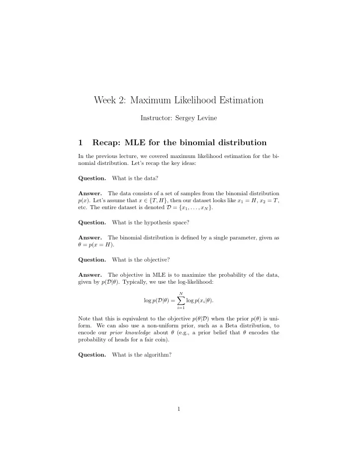
Week 2: Maximum Likelihood Estimation Instructor: Sergey Levine 1 Recap: MLE for the binomial distribution In the previous lecture, we covered maximum likelihood estimation for the bi- nomial distribution. Let’s recap the key ideas: What is the data? Question. The data consists of a set of samples from the binomial distribution Answer. p ( x ). Let’s assume that x ∈ { T, H } , then our dataset looks like x 1 = H , x 2 = T , etc. The entire dataset is denoted D = { x 1 , . . . , x N } . Question. What is the hypothesis space? Answer. The binomial distribution is defined by a single parameter, given as θ = p ( x = H ). Question. What is the objective? The objective in MLE is to maximize the probability of the data, Answer. given by p ( D| θ ). Typically, we use the log-likelihood: N � log p ( D| θ ) = log p ( x i | θ ) . i =1 Note that this is equivalent to the objective p ( θ |D ) when the prior p ( θ ) is uni- form. We can also use a non-uniform prior, such as a Beta distribution, to encode our prior knowledge about θ (e.g., a prior belief that θ encodes the probability of heads for a fair coin). What is the algorithm? Question. 1

Answer. The algorithm must solve the following problem ˆ θ ← arg max log p ( D| θ ) , θ (or p ( θ |D ) in the Bayesian case). We can solve this problem in the case of the binomial distribution by computing the derivative and setting it to zero. For more complex MLE problems, we might require a more sophisticated optimiza- tion algorithm. We’ll see some examples of this later in the class, but for now, let’s go through MLE for a different class of distributions. 2 Continuous data: Gaussian distributions What if instead of predicting whether the coin (or thumbtack...) will land heads or tails, we instead want to predict the probability that it will land at a particular point on the table (imagine for now that we only care about horizontal position – 1 dimension)? Now the variable x that we would like to model is real-valued. When dealing with real-valued random variables, one very popular choice of distribution is the Gaussian or Normal distribution, given by 1 2 π e − ( x − µ )2 p ( x | µ, σ ) = √ 2 σ 2 σ What is the hypothesis space if we want to model x using a Gaus- Question. sian distribution? The Gaussian is defined by two parameters: the mean µ and the Answer. standard deviation σ . Intuitively, µ corresponds to the “center” of the Gaussian, and σ corresponds to its width. The hypothesis space is fully defined by θ = { µ, σ } , where µ ∈ R and σ ∈ R + . A normally distributed random variable is typically written as x ∼ N ( µ, σ 2 ) . Gaussians have a few really useful properties that make them a popular choice for modeling continuous random variables. First, affine transformations of Gaussians are themselves Gaussian: if x ∼ N ( µ, σ 2 ), and y = ax + b , then y ∼ N ( aµ + b, a 2 σ 2 ). Second, the sum of two Gaussian random variables is also normally distributed: if x ∼ N ( µ x , σ 2 x ) and y ∼ N ( µ y , σ 2 y ), and z = x + y , then z ∼ N ( µ x + µ y , σ 2 x + σ 2 y ). There are also natural generalizations of the univari- ate normal distribution to the multivariate case, where � x is a multidimensional vector: in that case, µ is also a vector, and instead of the standard deviation σ , we use the covariance matrix Σ, which is a d × d matrix (where d is the dimensionality of � x ). But for now, let’s work with univariate Gaussians. Say that we record a dataset of samples from our (unknown) Gaussian, e.g. x 1 = 0 . 2, x 2 = 0 . 35, x 4 = 0 . 5, etc. Our goal is to learn the parameters µ and σ . 2

Like before, we can write the learning problem as N � µ, ˆ ˆ σ = arg max log p ( x i ) µ,σ i =1 Let’s derive the log likelihood: N N � 1 2 π e − ( xi − µ )2 � � � √ log p ( x i ) = log 2 σ 2 σ i =1 i =1 N 2 log 2 π − ( x i − µ ) 2 − log σ − 1 � = 2 σ 2 i =1 N ( x i − µ ) 2 � = − N log σ − + const . 2 σ 2 i =1 Now, let’s compute the optimal mean: � N � N ( x i − µ ) 2 ( x i − µ ) 2 d d � � − N log σ − + const = − dµ 2 σ 2 dµ 2 σ 2 i =1 i =1 N x i − µ � = = 0 σ 2 i =1 Rearranging the terms, we get: N σ 2 = N µ x i � σ 2 i =1 N 1 � x i = µ N i =1 This is the answer we expect: the optimal mean µ is the average value of all of our data points. Now let’s repeat the process for the standard deviation: � N � N ( x i − µ ) 2 � ( x i − µ ) 2 d = d d � � � − N log σ − dσ [ − N log σ ] − + const 2 σ 2 2 σ 2 dσ dσ i =1 i =1 N ( x i − µ ) 2 = − N � σ + = 0 σ 3 i =1 3

Rearranging, we get: N ( x i − µ ) 2 − N � σ + = 0 σ 3 i =1 N ( x i − µ ) 2 = Nσ 2 � i =1 N 1 ( x i − µ ) 2 = σ 2 � N i =1 Again, this is the equation we would expect for the variance, and the standard � � N 1 deviation is σ = i =1 ( x i − µ ) 2 . N 3 Bayesian learning with Gaussians Just like we did with the binomial distribution, we can also use Bayesian learning with Gaussian distributions. Question. What is the objective in Bayesian learning? The objective is the (log) probability of the parameters θ = { µ, σ } Answer. given the data: p ( θ |D ) ∝ p ( D| θ ) p ( θ ) log p ( θ |D ) = log p ( D| θ ) + log p ( θ ) + const For this exercise, let’s assume that we know the standard deviation σ , and we’re just trying to learn µ (we’ll see how to build a prior on σ later). The con- jugate prior for the mean of a Gaussian distribution is simply another Gaussian, with parameters µ 0 and σ 0 : − ( µ − µ 0)2 1 2 σ 2 p ( µ ) = √ 2 π e 0 σ 0 If we evaluate the posterior, we get: log p ( µ |D ) = log p ( D| µ ) + log p ( µ ) + const N ( x i − µ ) 2 − log σ 0 − ( µ − µ 0 ) 2 � = − N log σ − + const 2 σ 2 2 σ 2 0 i =1 Since all we want is a distribution over µ , we can fold any terms that don’t depend on µ into the constant (which we’ll figure out later), giving us N ( x i − µ ) 2 − ( µ − µ 0 ) 2 � log p ( µ |D ) = − + const 2 σ 2 2 σ 2 0 i =1 4

We can expand the quadratics in the numerators to get: i + µ 2 − 2 µx i − µ 2 + µ 2 N x 2 0 − 2 µ 0 µ � log p ( µ |D ) = − + const 2 σ 2 2 σ 2 0 i =1 N N x 2 − µ 2 2 σ 2 − µ 2 N 2 σ 2 − µ 2 1 2 x i + µ 2 µ 0 � � i 0 = − 2 σ 2 + µ + const 2 σ 2 2 σ 2 2 σ 2 0 0 0 i =1 i =1 � N � N � 1 � 2 σ 2 + 2 µ 0 2 x i � = − µ 2 2 σ 2 + + µ + const 2 σ 2 2 σ 2 0 0 i =1 Now, let � N � − 1 σ 2 + 1 σ 1 = σ 2 0 � N � σ 2 + µ 0 x i � µ 1 = σ 1 σ 2 0 i =1 We now have log p ( µ |D ) = − µ 2 + µµ 1 + const 2 σ 1 σ 1 = − µ 2 − 2 µµ 1 + const 2 σ 1 1 + µ 2 − 2 µµ 1 = − µ 2 + const 2 σ 1 = − ( µ − µ 1 ) 2 + const 2 σ 1 = − log σ 1 − 1 2 log 2 π − ( µ − µ 1 ) 2 + const 2 σ 1 The last line is precisely the equation for a Gaussian with mean µ 1 and standard deviation σ 1 . We know therefore that the constant on the last line is zero, because a Gaussian integrates to one, and therefore we have recovered the form of the posterior. It is again Gaussian. If we need to estimate the standard deviation σ , we typically put a prior instead on the variance σ 2 , and the conjugate prior is an inverse-gamma dis- tribution (you do not need to know this for homeworks or exams). This is a distribution over positive real numbers, and is given by β α � − β � Γ( α )( σ 2 ) − α − 1 exp p ( σ 2 ) = σ 2 If we need to estimate both σ and µ , we use the normal inverse-gamma dis- tribution, which is simply the product of a normal distribution on µ and an inverse-gamma on σ 2 . The posterior will be normal inverse-gamma. 5