Maximum Likelihood Estimation CS 446 Maximum likelihood: abstract - - PowerPoint PPT Presentation

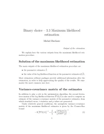
Maximum Likelihood Estimation

CS 446

Maximum likelihood: abstract formulation

We’ve had one main “meta-algorithm” this semester: ◮ (Regularized) ERM principle: pick the model that minimizes an average loss over training data.

1 / 70

Maximum likelihood: abstract formulation

We’ve had one main “meta-algorithm” this semester: ◮ (Regularized) ERM principle: pick the model that minimizes an average loss over training data. We’ve also discussed another: the “Maximum likelihood estimation (MLE)” principle: ◮ Pick a set of probability models for your data: P := {pθ : θ ∈ Θ}.

◮ pθ will denote both densities and masses; the literature is similarly inconsistent. ◮ Given samples (zi)n

i=1, pick the model that maximized the likelihood

max

θ∈Θ L(θ) = max θ∈Θ ln n

• i=1

pθ(zi) = max

θ∈Θ n

• i=1

ln pθ(zi), where the ln(·) is for mathematical convenience, and zi can be a labeled pair (xi, yi) or just xi.

1 / 70

Connections between ERM and MLE

◮ We can often derive and justify many basic methods with either (e.g., least squares, logistic regression, k-means, . . . ).

◮ MLE ideas were used to verive VAEs, which we’ll cover next week!

2 / 70

Connections between ERM and MLE

◮ We can often derive and justify many basic methods with either (e.g., least squares, logistic regression, k-means, . . . ).

◮ MLE ideas were used to verive VAEs, which we’ll cover next week!

◮ Each perspective suggests some different details and interpretation.

2 / 70

Connections between ERM and MLE

◮ We can often derive and justify many basic methods with either (e.g., least squares, logistic regression, k-means, . . . ).

◮ MLE ideas were used to verive VAEs, which we’ll cover next week!

◮ Each perspective suggests some different details and interpretation. ◮ Both approaches rely upon seemingly arbitrary assumptions and choices.

2 / 70

Connections between ERM and MLE

◮ We can often derive and justify many basic methods with either (e.g., least squares, logistic regression, k-means, . . . ).

◮ MLE ideas were used to verive VAEs, which we’ll cover next week!

◮ Each perspective suggests some different details and interpretation. ◮ Both approaches rely upon seemingly arbitrary assumptions and choices. ◮ The success of MLE seems to often hinge upon an astute choice of model.

◮ Applied scientists often like MLE and its ilk due to interpretability and “usability”: they can easily encode domain knowledge. We’ll return to this.

2 / 70

Example 1: coin flips.

◮ We flip a coin of bias θ ∈ [0, 1]. ◮ Write down xi = 0 for tails, xi = 1 for heads; then pθ(xi) = xiθ + (1 − xi)(1 − θ),

• r alternatively

pθ(xi) = θxi(1 − θ)1−xi. The second form will be more convenient.

3 / 70

Example 1: coin flips.

◮ We flip a coin of bias θ ∈ [0, 1]. ◮ Write down xi = 0 for tails, xi = 1 for heads; then pθ(xi) = xiθ + (1 − xi)(1 − θ),

• r alternatively

pθ(xi) = θxi(1 − θ)1−xi. The second form will be more convenient. ◮ Writing H :=

i xi and T := i(1 − xi) = n − H for convenience,

L(θ) =

n

• i=1
• xi ln θ + (1 − xi) ln(1 − θ)
• = H ln θ + T ln(1 − θ).

3 / 70

Example 1: coin flips.

◮ We flip a coin of bias θ ∈ [0, 1]. ◮ Write down xi = 0 for tails, xi = 1 for heads; then pθ(xi) = xiθ + (1 − xi)(1 − θ),

• r alternatively

pθ(xi) = θxi(1 − θ)1−xi. The second form will be more convenient. ◮ Writing H :=

i xi and T := i(1 − xi) = n − H for convenience,

L(θ) =

n

• i=1
• xi ln θ + (1 − xi) ln(1 − θ)
• = H ln θ + T ln(1 − θ).

Differentiating and setting to 0, 0 = H θ − T 1 − θ, which gives θ =

H T +H = H N .

◮ In this way, we’ve justified a natural algorithm.

3 / 70

Example 2: mean of a Gaussian

◮ Suppose xi ∼ N(µ, σ2), so θ = (µ, σ2), and ln pθ(xi) = ln exp

• − (xi−µ)2

2σ2

• √

2πσ2 = −(xi − µ)2 2σ2 − ln(2πσ2) 2 .

4 / 70

Example 2: mean of a Gaussian

◮ Suppose xi ∼ N(µ, σ2), so θ = (µ, σ2), and ln pθ(xi) = ln exp

• − (xi−µ)2

2σ2

• √

2πσ2 = −(xi − µ)2 2σ2 − ln(2πσ2) 2 . ◮ Therefore L(θ) = − 1 2σ2

n

• i=1

(xi − µ)2 + stuff without µ; applying ∇µ and setting to zero gives µ = 1 n

• i

xi. ◮ A similar derivation gives σ2 = 1

n

• i(xi − µ)2.

4 / 70

Discussion: Bayesian vs. frequentist perspectives

Question: n

i=1 xi n estimates a Gaussian µ parameter; but isn’t it useful

more generally?

5 / 70

Discussion: Bayesian vs. frequentist perspectives

Question: n

i=1 xi n estimates a Gaussian µ parameter; but isn’t it useful

more generally? Bayesian perspective: we choose a model and believe it well-approximates reality; learning its parameters determines underlying phenomena. ◮ Bayesian methods can handle model misspecification; LDA is an example which works well despite seemingly impractical assumptions.

5 / 70

Discussion: Bayesian vs. frequentist perspectives

Question: n

i=1 xi n estimates a Gaussian µ parameter; but isn’t it useful

more generally? Bayesian perspective: we choose a model and believe it well-approximates reality; learning its parameters determines underlying phenomena. ◮ Bayesian methods can handle model misspecification; LDA is an example which works well despite seemingly impractical assumptions. Frequentist perspective: we ask certain questions, and reason about the accuracy of our answers. ◮ For many distributions, n

i=1 xi n is a valid estimate of the mean,

moreover with confidence intervals of size 1/√n. This approach isn’t free of assumptions: IID is there. . .

5 / 70

Discussion: Bayesian vs. frequentist perspectives (part 2)

◮ Discussion also appears in the form “generative vs discriminative ML”. ◮ As before: both philosophies can justify/derive the same algorithm; they differ on some details (e.g., choosing k in k-means). ◮ IMO: it’s nice having more tools (as mentioned before: VAE derived from MLE perspective).

6 / 70

Example 3: Least squares (recap)

If we assume Y |X ∼ N(wTX, σ2), then L(w) =

n

• i=1

ln pw(xi, yi) =

n

• i=1
• ln pw(yi|xi) + ln p(xi)
• =

n

• i=1
• −(wTxi − yi)2

2σ2 + terms without w

• .

Therefore arg max

w∈Rd

L(w) = arg min

w∈Rd n

• i=1

(w

Txi − yi)2. 7 / 70

Example 3: Least squares (recap)

If we assume Y |X ∼ N(wTX, σ2), then L(w) =

n

• i=1

ln pw(xi, yi) =

n

• i=1
• ln pw(yi|xi) + ln p(xi)
• =

n

• i=1
• −(wTxi − yi)2

2σ2 + terms without w

• .

Therefore arg max

w∈Rd

L(w) = arg min

w∈Rd n

• i=1

(w

Txi − yi)2.

We can derive/justify the algorithm either way, but some refinements now differ with each perspective (e.g., regularization).

7 / 70

Example 4: Naive Bayes

◮ Let’s try a simple prediction setup, with (Bayes) optimal classifier arg max

y∈Y

p(Y = y|X = x). (We haven’t discussed this concept a lot, but it’s widespread in ML.)

8 / 70

Example 4: Naive Bayes

◮ Let’s try a simple prediction setup, with (Bayes) optimal classifier arg max

y∈Y

p(Y = y|X = x). (We haven’t discussed this concept a lot, but it’s widespread in ML.) ◮ One way to proceed is to learn p(Y |X) exactly; that’s a pain.

8 / 70

Example 4: Naive Bayes

◮ Let’s try a simple prediction setup, with (Bayes) optimal classifier arg max

y∈Y

p(Y = y|X = x). (We haven’t discussed this concept a lot, but it’s widespread in ML.) ◮ One way to proceed is to learn p(Y |X) exactly; that’s a pain. ◮ Let’s assume coordinates of X = (X1, . . . , Xd) are independent given Y : p(Y = y|X = x) = p(Y = y, X = x) p(X = x) = p(X = x|Y = y)p(Y = y) p(X = x) = p(Y = y) d

j=1 p(Xj = xj|Y = y)

p(X = x) , and arg max

y∈Y

p(Y = y|X = x) = arg max

y∈Y

p(Y = y)

d

• j=1

p(X = x)|Y = y).

8 / 70

Example 4: Naive Bayes (part 2)

arg max

y∈Y

p(Y = y|X = x) = arg max

y∈Y

p(Y = y)

d

• j=1

p(X = x)|Y = y).

9 / 70

Example 4: Naive Bayes (part 2)

arg max

y∈Y

p(Y = y|X = x) = arg max

y∈Y

p(Y = y)

d

• j=1

p(X = x)|Y = y). Examples where this helps: ◮ Suppose X ∈ {0, 1}d has an arbitrary distribution;\ it’s specified with 2d − 1 numbers.\ The factored form above needs d numbers. To see how this can help, suppose x ∈ {0, 1}d; instead of having to learn a probability model of 2d possibilities, we now have to learn d + 1 models each with 2 possibilities (binary labels). ◮ HW5 will use the standard “Iris dataset”.\ This data is continuous, Naive Bayes would approximate univariate distributions.

9 / 70

Mixtures of Gaussians.

10 / 70

k-means has spherical clusters?

Recall that k-means baked in spherical clusters. How about we model each cluster with a Gaussian?

11 / 70

k-means has spherical clusters?

Recall that k-means baked in spherical clusters.

5 5 10 15 10.0 7.5 5.0 2.5 0.0 2.5 5.0 7.5 10.0

How about we model each cluster with a Gaussian?

11 / 70

k-means has spherical clusters?

Recall that k-means baked in spherical clusters.

5 5 10 15 10.0 7.5 5.0 2.5 0.0 2.5 5.0 7.5 10.0

How about we model each cluster with a Gaussian?

11 / 70

k-means has spherical clusters?

Recall that k-means baked in spherical clusters.

5 5 10 15 10.0 7.5 5.0 2.5 0.0 2.5 5.0 7.5 10.0

How about we model each cluster with a Gaussian?

11 / 70

k-means has spherical clusters?

Recall that k-means baked in spherical clusters.

5 5 10 15 10.0 7.5 5.0 2.5 0.0 2.5 5.0 7.5 10.0

How about we model each cluster with a Gaussian?

11 / 70

k-means has spherical clusters?

Recall that k-means baked in spherical clusters.

5 5 10 15 10.0 7.5 5.0 2.5 0.0 2.5 5.0 7.5 10.0

How about we model each cluster with a Gaussian?

11 / 70

k-means has spherical clusters?

Recall that k-means baked in spherical clusters.

5 5 10 15 10.0 7.5 5.0 2.5 0.0 2.5 5.0 7.5 10.0

How about we model each cluster with a Gaussian?

11 / 70

k-means has spherical clusters?

Recall that k-means baked in spherical clusters.

5 5 10 15 10.0 7.5 5.0 2.5 0.0 2.5 5.0 7.5 10.0

How about we model each cluster with a Gaussian?

11 / 70

k-means has spherical clusters?

Recall that k-means baked in spherical clusters.

5 5 10 15 10.0 7.5 5.0 2.5 0.0 2.5 5.0 7.5 10.0

How about we model each cluster with a Gaussian?

11 / 70

k-means has spherical clusters?

Recall that k-means baked in spherical clusters.

5 5 10 15 10.0 7.5 5.0 2.5 0.0 2.5 5.0 7.5 10.0

How about we model each cluster with a Gaussian?

11 / 70

Gaussian Mixture Model

◮ Suppose data is drawn from k Gaussians, meaning Y = j ∼ Discrete(π1, . . . , πk), X = x|Y = j ∼ N(µj, Σj), and the parameters are θ = ((π1, µ1, Σ1), . . . , (πk, µk, Σk)). (Note: this is a generative model, and we have a way to sample.) ◮ The probability density at a given x is pθ(x) =

k

• j=1

pµj,Σj(x|Y = j)πj, and the maximum likelihood problem becomes

L((πj, µj, Σj)k

j=1) = n

• i=1

ln

k

• j=1

πj

• (2π)d|Σ|

exp

• −1

2(xi − µj)

TΣ−1(xi − µj)

• The ln and the exp are no longer next to each other; we can’t just

take the derivative and set the answer to 0.

12 / 70

Pearson’s crabs.

Statistician Karl Pearson wanted to understand the distribution of “forehead breadth to body length” for 1000 crabs

0.58 0.60 0.62 0.64 0.66 0.68 5 10 15 20 25

13 / 70

Pearson’s crabs.

Statistician Karl Pearson wanted to understand the distribution of “forehead breadth to body length” for 1000 crabs

0.58 0.60 0.62 0.64 0.66 0.68 5 10 15 20 25

Doesn’t look Gaussian!

13 / 70

Pearson’s crabs.

Statistician Karl Pearson wanted to understand the distribution of “forehead breadth to body length” for 1000 crabs

0.58 0.60 0.62 0.64 0.66 0.68 5 10 15 20 25

Pearson fit a mixture of two Gaussians.

14 / 70

Pearson’s crabs.

Statistician Karl Pearson wanted to understand the distribution of “forehead breadth to body length” for 1000 crabs

0.58 0.60 0.62 0.64 0.66 0.68 5 10 15 20 25

Pearson fit a mixture of two Gaussians.

• Remark. Pearson did not use E-M. For this he invented the “method of

moments” and obtained a solution by hand.

14 / 70

Aside: why Gaussians at all?

◮ You can argue Gaussian is a good model for single populations thanks to the CLT (Central Limit Theorem). ◮ Pearson, seeing the skewed distribution, felt there are two populations. ◮ Treating these populations as independent,

• ne gets a mixture of Gaussians.

15 / 70

Summary of part 1.

16 / 70

Summary (of part 1)

◮ MLE principle; its philosophy and when it might work well. ◮ Naive Bayes. ◮ The generative model of Gaussian Mixtures.

17 / 70