Class 2 & 3 Overfitting & Regularization Carlo Ciliberto - PowerPoint PPT Presentation
Class 2 & 3 Overfitting & Regularization Carlo Ciliberto Department of Computer Science, UCL October 18, 2017 Last Class The goal of Statistical Learning Theory is to find a good estimator f n : X Y , approximating the lowest
Class 2 & 3 Overfitting & Regularization Carlo Ciliberto Department of Computer Science, UCL October 18, 2017
Last Class The goal of Statistical Learning Theory is to find a “good” estimator f n : X → Y , approximating the lowest expected risk � f : X→Y E ( f ) , E ( f ) = inf ℓ ( f ( x ) , y ) dρ ( x, y ) X×Y given only a finite number of (training) examples ( x i , y i ) n i =1 sampled independently from the unknown distribution ρ .
Last Class: The SLT Wishlist What does “good” estimator mean? Low excess risk E ( f n ) − E ( f ∗ ) ◮ Consistency . Does E ( f n ) − E ( f ∗ ) → 0 as n → + ∞ – in Expectation? – in Probability? with respect to a training set S = ( x i , y i ) n i =1 of points randomly sampled from ρ . ◮ Learning Rates . How “fast” is consistency achieved? Nonasymptotic bounds: finite sample complexity, tail bounds, error bounds...
Last Class (Expected Vs Empirical Risk) Approximate the expected risk of f : X → Y via its empirical risk n E n ( f ) = 1 � ℓ ( f ( x i ) , y i ) n i =1 � V f ◮ Expectation: E |E n ( f ) − E ( f ) | ≤ n ◮ Probability (e.g. using Chebyshev): P ( |E n ( f ) − E ( f ) | ≥ ǫ ) ≤ V f ∀ ǫ > 0 nǫ 2 where V f = Var ( x,y ) ∼ ρ ( ℓ ( f ( x ) , y )) .
Last Class (Empirical Risk Minimization) Idea : if E n is a good approximation to E , then we could use E n ( f ) f n = argmin f ∈F to approximate f ∗ . This is known as empirical risk minimization (ERM) Note : If we sample the points in S = ( x i , y i ) n i =1 independently from ρ , the corresponding f n = f S is a random variable and we have E E ( f n ) − E ( f ∗ ) ≤ E E ( f n ) − E n ( f n ) Question : does E E ( f n ) − E n ( f n ) go to zero as n increases?
Issues with ERM Assume X = Y = R , ρ with dense support 1 and ℓ ( y, y ) = 0 ∀ y ∈ Y . For any set ( x i , y i ) n i =1 s.t. x i � = x j ∀ i � = j let f n : X → Y be such that � if x = x i ∃ i ∈ { 1 , . . . n } y i f n ( x ) = 0 otherwise Then, for any number n of training points: ◮ E E n ( f n ) = 0 ◮ E E ( f n ) = E (0) , which is greater than zero (unless f ∗ ≡ 0 ) Therefore E E ( f n ) − E n ( f n ) = E (0) � 0 as n increases! 1 and such that every pair ( x, y ) has measure zero according to ρ
Overfitting An estimator f n is said to overfit the training data if for any n ∈ N : ◮ E E ( f n ) − E ( f ∗ ) > C for a constant C > 0 , and ◮ E E n ( f n ) − E n ( f ∗ ) ≤ 0 According to this definition ERM overfits...
ERM on Finite Hypotheses Spaces Is ERM hopeless? Consider the case X and Y finite. Then, F = Y X = { f : X → Y} is finite as well (albeit possibly large), and therefore: E |E n ( f n ) − E ( f n ) | ≤ E sup |E n ( f ) − E ( f ) | f ∈F � � ≤ E |E n ( f ) − E ( f ) | ≤ |F| V F /n f ∈F where V F = sup f ∈F V f and |F| denotes the cardinality of F . Then ERM works! Namely: lim n → + ∞ E |E ( f n ) − E ( f ) | = 0
ERM on Finite Hypotheses (Sub) Spaces The same argument holds in general: let H ⊂ F be a finite space of hypotheses. Then, � E |E n ( f n ) − E ( f n ) | ≤ |H| V H /n In particular, if f ∗ ∈ H , then � E |E ( f n ) − E ( f ∗ ) | ≤ |H| V H /n and ERM is a good estimator for the problem considered.
Example: Threshold functions Consider a binary classification problem Y = { 0 , 1 } . Someone has told us that the minimizer of the risk is a “threshold function” f a ∗ ( x ) = 1 [ a ∗ , + ∞ ) with a ∗ ∈ [ − 1 , 1] . 1.5 a b 1 0.5 0 -1.5 -1 -0.5 0 0.5 1 1.5 We can learn on H = { f a | a ∈ R } = [ − 1 , 1] . However on a computer we can only represent real numbers up to a given precision .
Example: Threshold Functions (with precision p ) Discretization : given a p > 0 , we can consider H p = { f a | a ∈ [ − 1 , 1] , a · 10 p = [ a · 10 p ] } with [ a ] denoting the integer part (i.e. the closest integer) of a scalar a . The value p can be interpreted as the “precision” of our space of functions H p . Note that |H p | = 2 · 10 p If f ∗ ∈ H p , then we have automatically that V H /n ≤ 10 p / √ n � E |E ( f n ) − E ( f ∗ ) | ≤ |H p | ( V H ≤ 1 since ℓ is the 0 - 1 loss and therefore | ℓ ( f ( x ) , y ) | ≤ 1 for any f ∈ H )
Rates in Expectation Vs Probability In practice, even for small values of p E |E ( f n ) − E ( f ∗ ) | ≤ 10 p / √ n will need a very large n in order to have a meaningful bound on the expected error. Interestingly, we can get much better constants (not rates though!) by working in probability...
Hoeffding’s Inequality Let X 1 , . . . , X n independent random variables s.t. X i ∈ [ a i , b i ] . � n Let X = 1 i =1 X i . Then, n � � 2 n 2 ǫ 2 �� � � � ≥ ǫ � X − E X ≤ 2 exp − P � n i =1 ( b i − a i ) 2
Applying Hoeffding’s inequality Assume that ∀ f ∈ H , x ∈ X , y ∈ Y the loss is bounded | ℓ ( f ( x ) , y ) | ≤ M by some constant M > 0 . Then, for any f ∈ H we have P ( |E n ( f ) − E ( f ) | ≥ ǫ ) ≤ exp( − nǫ 2 2 M 2 )
Controlling the Generalization Error We would like to control the generalization error E n ( f n ) − E ( f n ) of our estimator in probability . One possible way to do that is by controlling the generalzation error of the whole set H . � � P ( |E n ( f n ) − E ( f n ) | ≥ ǫ ) ≤ P sup |E n ( f ) − E ( f ) | ≥ ǫ f ∈H The latter term is the probability that least one of the events |E n ( f ) − E ( f ) | ≥ ǫ occurs for f ∈ H . In other words the probability of the union of such events. Therefore � � � sup |E n ( f ) − E ( f ) | ≥ ǫ ≤ P ( |E n ( f ) − E ( f ) | ≥ ǫ ) P f ∈H f ∈H by the so-called union bound .
Hoeffding the Generalization Error By applying Hoeffding’s inequality, P ( |E n ( f n ) − E ( f n ) | ≥ ǫ ) ≤ 2 |H| exp( − nǫ 2 2 M 2 ) Or, equivalently, that for any δ ∈ (0 , 1] , � 2 M 2 log(2 |H| /δ ) |E n ( f n ) − E ( f n ) | ≤ n with probability at least 1 − δ .
Example: Threshold Functions (in Probability) Going back to H p space of threshold functions... � 4 + 6 p − 2 log δ |E n ( f n ) − E ( f n ) | ≤ n since M = 1 and log 2 |H| = log 4 · 10 p = log 4 + p log 10 ≤ 2 + 3 p . For example, let δ = 0 . 001 . We can say that � 6 p + 18 |E n ( f n ) − E ( f n ) | ≤ n holds at least 99 . 9% of the times.
Bounds in Expectation Vs Probability Comparing the two bounds E |E n ( f n ) − E ( f n ) | ≤ 10 p / √ n (Expectation) While, with probability greater than 99 . 9% � 6 p + 18 |E n ( f n ) − E ( f n ) | ≤ (Probability) n Although we cannot be 100% sure of it, we can be quite confident that the generalization error will be much smaller than what the bound in expectation tells us... Rates : note however that the rates of convergence to 0 are the same (i.e. O (1 / √ n ) ).
Improving the bound in Expectation Exploiting the bound in probability and the knowledge that on H p the excess risk is bounded by a constant, we can improve the bound in expectation... Let X be a random variable s.t. | X | < M for some constant M > 0 . Then, for any ǫ > 0 we have E | X | ≤ ǫ P ( | X | ≤ ǫ ) + M P ( | X | > ǫ ) Applying to our problem: for any δ ∈ (0 , 1] � 2 M 2 log(2 |H p | /δ ) E |E n ( f n ) − E ( f n ) | ≤ (1 − δ ) + δM n Therefore only log |H p | appears (no |H p | alone).
Infinite Hypotheses Spaces What if f ∗ ∈ H \ H p for any p > 0 ? ERM on H p will never minimize the expected risk. There will always be a gap for E ( f n,p ) − E ( f ∗ ) . For p → + ∞ it is natural to expect such gap to decrease... BUT if p increases too fast (with respect to the number n of examples) we cannot control the generalization error anymore! � 6 p + 18 |E n ( f n ) − E ( f n ) | ≤ → + ∞ for p → + ∞ n Therefore we need to increase p gradually as a function p ( n ) of the number of training examples. This approach is known as regularization .
Approximation Error for Threshold Functions Let’s consider f p = 1 [ a p , + ∞ ) argmin f ∈ H p E ( f ) with a p ∈ [ − 1 , 1] . Consider the error decomposition of the excess risk E ( f n ) − E ( f ∗ ) : E ( f n ) − E n ( f n ) + E n ( f n ) − E n ( f p ) + E n ( f p ) − E ( f p ) + E ( f p ) − E ( f ∗ ) � �� � ≤ 0 We already know how to control the generalization of f n (via the supremum over H p ) and f p (since it is a single function). Moreover, we have that the approximation error is E ( f p ) − E ( f ∗ ) ≤ | a p − a ∗ | ≤ 10 − p (why?) Note that it does not depend on training data!
Approximation Error for Threshold Functions II Putting everything together we have that, for any δ ∈ [0 , 1) and p ≥ 0 , � 4 + 6 p − 2 log δ + 10 − p = φ ( n, δ, p ) E ( f n ) − E ( f ∗ ) ≤ 2 n holds with probability greater or equal to 1 − δ . In particular, for any n and δ , we can choose the best precision as p ( n, δ ) = argmin φ ( n, δ, p ) p ≥ 0 which leads to an error bound ǫ ( n, δ ) = φ ( n, δ, p ( n, δ )) holding with probability larger or equal than 1 − δ .
Recommend
More recommend
Explore More Topics
Stay informed with curated content and fresh updates.
