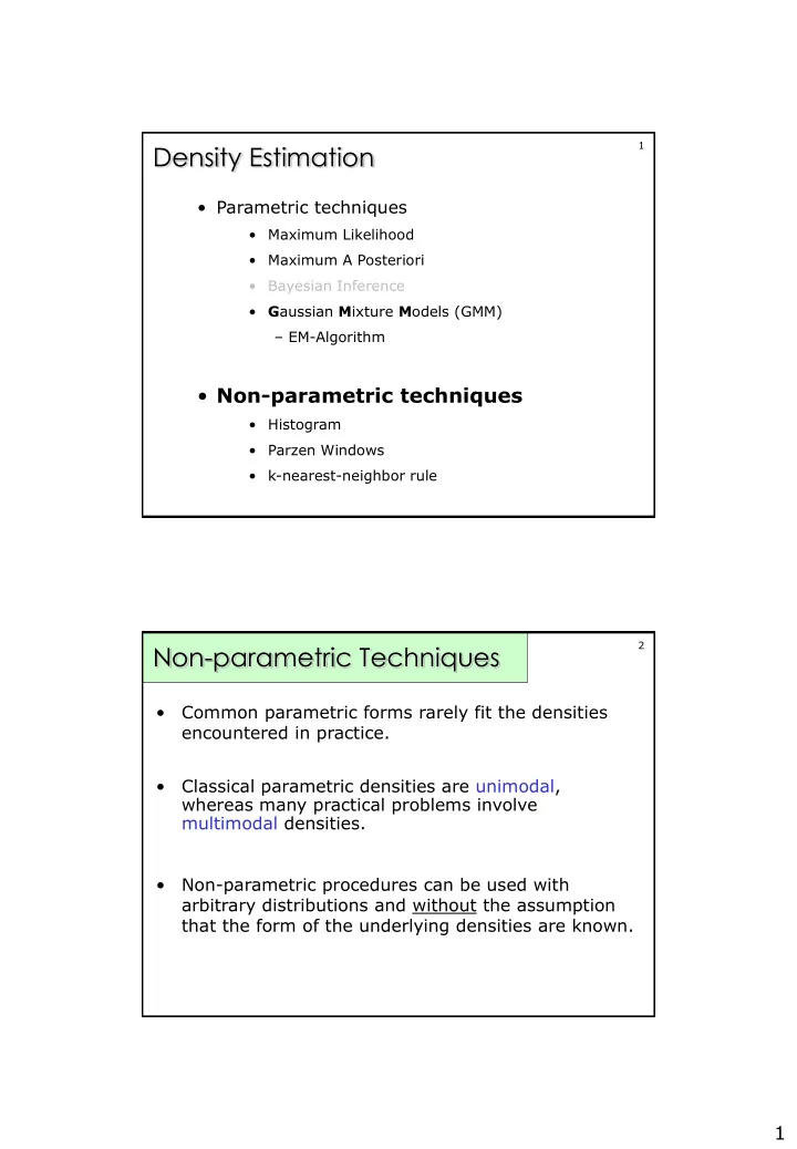
Density Estimation Parametric techniques Maximum Likelihood - PDF document

1 Density Estimation • Parametric techniques • Maximum Likelihood • Maximum A Posteriori • Bayesian Inference • G aussian M ixture M odels (GMM) – EM-Algorithm • Non-parametric techniques • Histogram • Parzen Windows • k-nearest-neighbor rule 2 Non-parametric Techniques • Common parametric forms rarely fit the densities encountered in practice. • Classical parametric densities are unimodal, whereas many practical problems involve multimodal densities. • Non-parametric procedures can be used with arbitrary distributions and without the assumption that the form of the underlying densities are known. 1

3 Histograms • Conceptually most simple and intuitive method to estimate a p.d.f. is a histogram. • The range of each dimension x i of vector x is divided into a fixed number m of intervals. • The resulting M boxes (bins) of identical volume V count the number of points falling into each bin: • Assume we have N samples ( x i ) and the number of points x l in the j-th bin, b j , is k j . Then the histogram estimate of the density is: / k N   j ( ) , p x x b j V 4 Histograms ( ) p x • … is constant over every bin b j • … is a density function M M k 1        j p ( x ) dx dx k 1 j b NV N  j  1 1 j j • The number of bins M and their starting positions are “parameters”. However only the choice of M is critical. It plays the role of a smoothing parameter. 2

5 Histograms: Example • Assume one dimensional data sampled from a combination of two Gaussians • 3 bins 6 Histograms: Example • 7 bins • 11 bins 3

7 Histogram Approach • Histogram p.d.f. estimator is very efficient since it can be computed online ( only update counters, no need to keep all data ) • Usefulness is limited to low dimensional vectors, since number of bins, M , grows exponentially with data’s dimensionality d : M= m d  “Curse of dimensionality” 8 Parzen Windows: Motivation • Consider set of 1-D samples { x 1 , …, x N } of which we want to estimate the density • We can easily get estimate of cumulative distribution function (CDF) as:  #(samples) x  ( ) P x N • Density p(x ) is the derivative of the CDF • But that is discontinuous !! 4

9 Parzen Windows: • What we can do, is to estimate the density as:  h   h P x ( ) P x ( ) 2 2   ( ) , 0 p x h h • This is the proportion of observations falling within the interval [ x-h/2 , x+h/2 ] divided by h . • We can rewrite the estimate (already for d dim .):    N 1 x x   i ( ) x p K   d   Nh h  i 1      1 z 1 1... j d 2 with   j ( ) K z   0 otherwise 10 Parzen Windows: • The resulting density estimate itself is not continuous. • This is because points within a distance h/2 of x contribute a value 1/N to the density and points further away a value of zero. • Idea to overcome this limitation: Generalize the estimator by using a smoother weighting function (e.g. one that decreases as | z | increases). This weighting function K is termed kernel and the parameter h is the spread (or bandwidth ). 5

11 Parzen Windows • The kernel is used for interpolation: each sample contributes to the estimate according to its distance from x • For a density, must: p x ( ) - Be non-negative - Integrate to 1 • This can be assured by requiring the kernel itself to fulfill the requirements of a density function, ie.:        ( ) 0 and ( ) z z 1 K x K d 12 Parzen Windows: Kernels Discontinuous Kernel Functions :    0 x 1 Rectangular:   2 ( ) x K   1 x 1  2 Triangular:    0 x 1    ( x ) K   1 x x 1  Smooth Kernels: Normal:   2 1 x ( ) exp( ) K x  2 2 Multivariate normal:   d  T x x ( ) x  exp( ) K 2 (2 ) (radially symm. univ. Gaussian) 2 6

13 Parzen Windows: Bandwidth • The choice of bandwidth is critical ! Examples of two-dimensional circularly symmetric normal Parzen windows for 3 different values of h . 14 Parzen Windows: Bandwidth 3 Parzen-window density estimates based on the same set of 5 samples, using windows from previous figure If h is too large the estimate will suffer from too little  resolution. If h is too small the estimate will suffer from too much  statistical variability. 7

15 Parzen Windows: Bandwidth • The decision regions of a PW-classifier also depend on bandwidth (and of course of kernel). Small h : more complicated Large h : less complicated boundaries boundaries 16 k-Nearest-Neighbor Estimation • Similar to histogram approach. • Estimate from N training samples by centering p x ( ) a volume V around x and letting it grow until it captures k samples. These samples are the k nearest neighbors of x . • • In regions of high density (around x ) the volume will be relatively small. • k plays a similar role as the bandwidth parameter in PW. 8

17 • Let N be the total number of samples and V the volume around x which contains k samples then k  ( ) x p  ( ) N V x k-NN Decision Rule (Classifier) • Suppose that in the k samples we find k m from class  m (so that ).  M  k k  m m 1 • Let the total number of samples in class  m be n m (so that ) .  M  n N  m m 1 18 k-NN Decision Rule (Classifier) • Then we may estimate the class-conditional density p ( x |  m ) as k   m ( x | ) p m n V m and the prior probability p (  m ) as n   m p ( ) m N • Using these estimates the decision rule:     assign x to  m if : ( | x ) ( | x ) i p p m i translates (Bayes’ theorem) to: assign x to  m if   : i k k m i 9

19 k-NN Decision Rule (Classifier)  The decision rule is to assign x to the class that receives the largest vote amongst the k nearest neighbors of all classes M . • For k=1 this is the nearest neighbor rule producing a Voronoi- tesselation of the training space. • This rule is sub-optimal, but when the number of prototypes is large, its error is never worse than twice the Bayes error classification probability P B . M     P P P (2 P ) 2 P B kNN B  B B 1 M 20 Non-parametric comparison • Parzen window estimates require storage of all observations and n evaluations of the kernel function for each estimate, which is computationally expensive! • Nearest neighbor requires the storage of all the observations. • Histogram estimates do not require storage for all the observations, they require storage for the description of the bins. But for simple histograms the number of the bins grows exponentially with the dimension of the observation space. 10

21 Non-parametric Techniques Advantages • Generality: same procedure for unimodal, normal and bimodal mixture. • No assumption about the distribution required ahead of time. • With enough samples we can converge to an arbitrarily complicated target density. 22 Non-parametric Techniques Disadvantages • Number of required samples may be very large (much larger than would be required if we knew the form of the unknown density) . • Curse of dimensionality. • In case of PW and KNN computationally expensive (storage & processing). • Sensitivity to choice of bin size, bandwidth,… 11