Lecture 4. Maximum Likelihood Estimation - confidence intervals. - PowerPoint PPT Presentation
Lecture 4. Maximum Likelihood Estimation - confidence intervals. Igor Rychlik Chalmers Department of Mathematical Sciences Probability, Statistics and Risk, MVE300 Chalmers April 2013. Click on red text for extra material. Maximum
Lecture 4. Maximum Likelihood Estimation - confidence intervals. Igor Rychlik Chalmers Department of Mathematical Sciences Probability, Statistics and Risk, MVE300 • Chalmers • April 2013. Click on red text for extra material.
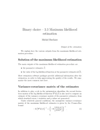
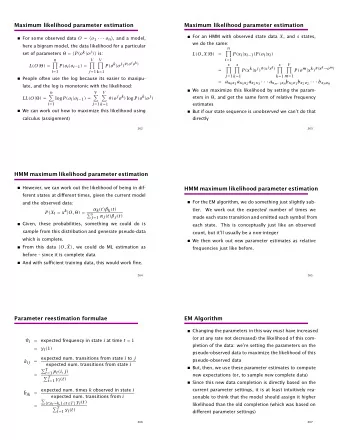
Maximum Likelihood method It is parametric estimation procedure of F X consisting of two steps: choice of a model ; finding the parameters : ◮ Choose a model, i.e. select one of the standard distributions F ( x ) (normal, exponential, Weibull, Poisson ...). Next postulate that � x − b � F X ( x ) = F . a ◮ Find estimates ( a ∗ , b ∗ ) such that F X ( x ) ≈ F � ( x − b ∗ ) / a ∗ � . The maximum likelihood estimates ( a ∗ , b ∗ ) will be presented.
Finding likelihood, review from Lecture 1: ◮ Let A 1 , A 2 , . . . , A k be a partition of the sample space, i.e. k excluding alternatives such that one of them is true. Suppose that it is equally probable that any of A i is true, i.e. prior odds q 0 i = 1. ◮ Let B 1 , . . . , B n be true statements (evidences) and let B be the event that all B i are true, i.e. B = B 1 ∩ B 2 ∩ . . . ∩ B n . ◮ The new odds q n i for A i after collecting B i evidences are q n i = P( B | A i ) · q 0 i = P( B | A i ) · 1 = P ( B 1 | A i ) · . . . · P ( B n | A i ) . Function L ( A i ) = P( B | A i ) is called likelihood that A i is true.
The ML estimate - discrete case: The maximum likelihood method recommends to choose the alternative A ∗ i having highest likelihood, i.e. find i for which the likelihood L ( A i ) is highest. Example 1 Binomial cdf. 0.16 0.14 0.12 0.1 L( θ ) 0.08 0.06 0.04 θ * 0.02 0 0 0.2 0.4 0.6 0.8 1 θ
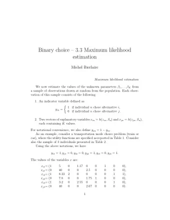
ML estimate - continuous variable: Model : Let consider a continuous rv. and postulate that F X ( x ) is exponential cdf, i.e. F X ( x ) = 1 − exp( − x / a ) and pdf f X ( x ) = exp( − x / a ) / a = f ( x ; a ) . Data : x = ( x 1 , x 2 , . . . , x n ) are observations of X . (Example: the earthquake data where n = 62 obs.) Likelihood function : 1 In practice data is given with finite number of digits, hence one only knows that events B i =” x i − ǫ < X ≤ x i + ǫ ” is true. For small ǫ , P( B i ) ≈ f X ( x i ) · 2 ǫ thus L ( a ) = P( B 1 | a ) · . . . · P( B n | a ) = (2 ǫ ) n f ( x 1 ; a ) · . . . · f ( x n ; a ) . ML-estimate : a ∗ maximizes L ( a ) or log-likelihood l ( a ) = ln L ( a ). Example 2 Exponential cdf. 1 Since P( X = x i ) = 0 for all values of parameter a it is not obvious how to define the likelihood function L ( a ).
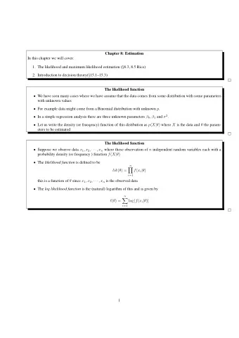
Sumarizing - Maximum Likelihood Method. For n independent observations x 1 , . . . , x n the likelihood function � f ( x 1 ; θ ) · f ( x 2 ; θ ) · . . . · f ( x n ; θ ) (continuous r.v.) L ( θ ) = p ( x 1 ; θ ) · p ( x 2 ; θ ) · . . . · p ( x n ; θ ) (discrete r.v.) where f ( x ; θ ), p ( x ; θ ) is probability density and probability-mass function, respectively. The value of θ which maximizes L ( θ ) is denoted by θ ∗ and called the ML estimate of θ . Example 3 Censored data.
Example: Estimation Error E Suppose that position of moving equipment is measured periodically using GPS. Example of sequence of positions p GPS is 1.16, 2.42, 3.55, ..., km. Calibration procedure of the GPS states that the error E = p true − p GPS is approximately normal; is in average zero (no bias) and has standard deviation σ = 50 meters. What does it means in practice? Quantiles of the standard normal distribution. α 0.10 0.05 0.025 0.01 0.005 0.001 λ α 1.28 1.64 1.96 2.33 2.58 3.09 Example 4 e α = σλ α .
Confidence interval: Clearly error E = p true − p GPS is with probability 1 − α in the interval: P( e 1 − α/ 2 ≤ E ≤ e α/ 2 ) = 1 − α. For α = 0 . 05, e α/ 2 ≈ 1 . 96 σ , e 1 − α/ 2 ≈ − 1 . 96 σ , σ = 50 m, hence p GPS − 1 . 96 · 50 ≤ p true ≤ p GPS + 1 . 96 · 50 � � 1 − α ≈ P p true ∈ [ p GPS − 1 . 96 · 50 , p GPS + 1 . 96 · 50] � � = P . ★ ✥ If we measure many times positions using the same GPS and errors are inde- pendent then frequency of times statement A = ” p true ∈ [ p GPS − 1 . 96 · 50 , p GPS + 1 . 96 · 50]” ✧ ✦ is true will be close to 0 . 95. 2 2 Often, after observing an outcome of an experiment, one can tell whether a statement about outcome is true or not. Observe that this is not possible for A !
Asymptotic normality of error E : When unknown parameter θ , say, is estimated by mean of observations then by Central Limit Theorem the error E = θ − θ ∗ has mean zero and is asymptotically (as number of observations n tends to infinity) normally distributed. 3 ( σ 2 E ) ∗ Distribution ML estimates θ ∗ θ ∗ = ¯ X ∈ Po( θ ) x n θ ∗ (1 − θ ∗ ) θ ∗ = k K ∈ Bin( n , θ ) n n ( θ ∗ ) 2 θ ∗ = ¯ X ∈ Exp( θ ) x n s 2 θ ∗ = ¯ X ∈ N( θ, σ 2 ) n x n Example 5 3 Similar result was valid for GPS estimates of positions.
Confidence interval for unknown parameter: As for GPS measurements, probability that statement A = ” θ ∈ [ θ ∗ − λ α/ 2 σ ∗ E , θ ∗ + λ α/ 2 σ ∗ E ]” , is true is approximately 1 − α . Since we can not tell whether A is true or not the probability measures lack of knowledge . Hence one call the probability confidence 4 . ✬ ✩ Under some assumptions, the ML estimation error E = θ − θ ∗ is asymp- � − ¨ totically normal distributed. With σ ∗ E = 1 / l ( θ ∗ ) θ ∈ [ θ ∗ − λ α/ 2 σ ∗ E , θ ∗ + λ α/ 2 σ ∗ E ] , ✫ ✪ with approximately 1 − α confidence. 4 However if we use confidence intervals to measure uncertainty of estimated parameters values then in long run the statements A will be true with 1 − α frequency
Example - Earthquake data: Recall - the ML-estimate is a ∗ = 437 . 2 days and, with the α = 0 . 05, √ √ e 1 − α/ 2 = − 1 . 96 · 3083 = − 108 . 8 , e α/ 2 = 1 . 96 · 3083 = 108 . 8 . and hence, with approximate confidence 1 − α , a ∈ [437 . 25 − 108 . 8 , 437 . 2 + 108 . 8] = [328 , 546] . For exponential distribution with parameter a there is also exact interval: with confidence 1 − α � � 2 na ∗ 2 na ∗ θ ∈ α/ 2 (2 n ) , , χ 2 χ 2 1 − α/ 2 (2 n ) where χ 2 α ( f ) is the α quantile of the χ 2 ( f ) distribution. For the data α = 0 . 05, n = 62, χ 2 1 − α/ 2 (2 n ) = 95 . 07, χ 2 α/ 2 (2 n ) = 156 . 71 gives a ∈ [346 , 570] .
Example - normal cdf: Suppose we have independent observations x 1 , . . . , x n from N( m , σ 2 ), σ unknown . Here one can construct an exact interval for m , viz. estimate σ 2 by n 1 ( σ 2 ) ∗ = x ) 2 = s 2 � ( x i − ¯ n − 1 , n − 1 i =1 then the exact confidence interval for m is given by � � x − t α/ 2 ( n − 1) s n − 1 x + t α/ 2 ( n − 1) s n − 1 ¯ √ n , ¯ √ n where t α/ 2 ( f ) are quantiles of the so-called Student’s t distribution with f = n − 1 degrees of freedom. The asymptotic interval is � � s n s n x − λ α/ 2 ¯ √ n , ¯ x + λ α/ 2 √ n . Consider α = 0 . 05. Then λ α/ 2 = 1 . 96 and for n = 10, one has t α/ 2 (9) = 2 . 26 while for n = 25, t α/ 2 (24) = 2 . 06, which is closer to λ α/ 2 = 1 . 96.
Recommend
More recommend
Explore More Topics
Stay informed with curated content and fresh updates.
