Confidence intervals for the mixing time of a reversible Markov - PowerPoint PPT Presentation

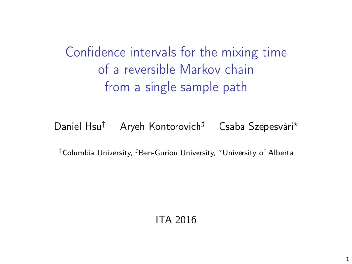
Confidence intervals for the mixing time of a reversible Markov chain from a single sample path Daniel Hsu † Aryeh Kontorovich ♯ Csaba Szepesvári ⋆ † Columbia University, ♯ Ben-Gurion University, ⋆ University of Alberta ITA 2016 1

Problem ◮ Irreducible, aperiodic, time-homogeneous Markov chain X 1 → X 2 → X 3 → · · · 2

Problem ◮ Irreducible, aperiodic, time-homogeneous Markov chain X 1 → X 2 → X 3 → · · · ◮ There is a unique stationary distribution π with t →∞ L ( X t | X 1 = x ) = π , lim for all x ∈ X . 2

Problem ◮ Irreducible, aperiodic, time-homogeneous Markov chain X 1 → X 2 → X 3 → · · · ◮ There is a unique stationary distribution π with t →∞ L ( X t | X 1 = x ) = π , lim for all x ∈ X . ◮ The mixing time t mix is the earliest time t with sup �L ( X t | X 1 = x ) − π � tv ≤ 1 / 4 . x ∈X 2

Problem ◮ Irreducible, aperiodic, time-homogeneous Markov chain X 1 → X 2 → X 3 → · · · ◮ There is a unique stationary distribution π with t →∞ L ( X t | X 1 = x ) = π , lim for all x ∈ X . ◮ The mixing time t mix is the earliest time t with sup �L ( X t | X 1 = x ) − π � tv ≤ 1 / 4 . x ∈X Problem : Determine (confidently) if t ≥ t mix after seeing X 1 , X 2 , . . . , X t . 2

Problem ◮ Irreducible, aperiodic, time-homogeneous Markov chain X 1 → X 2 → X 3 → · · · ◮ There is a unique stationary distribution π with t →∞ L ( X t | X 1 = x ) = π , lim for all x ∈ X . ◮ The mixing time t mix is the earliest time t with sup �L ( X t | X 1 = x ) − π � tv ≤ 1 / 4 . x ∈X Problem : Given δ ∈ ( 0 , 1 ) and X 1 : t , determine non-trivial I t ⊆ [ 0 , ∞ ] with P ( t mix ∈ I t ) ≥ 1 − δ . 2

Some motivation from machine learning and statistics Chernoff bounds for Markov chains X 1 → X 2 → · · · : for suitably well-behaved f : X → R , with probability at least 1 − δ , � � �� � � � t � � � 1 t mix log ( 1 /δ ) � � ˜ f ( X i ) − E π f ≤ O . � � t t � � i = 1 � �� � deviation bound Bound depends on t mix , which may be unknown a priori . 3

Some motivation from machine learning and statistics Chernoff bounds for Markov chains X 1 → X 2 → · · · : for suitably well-behaved f : X → R , with probability at least 1 − δ , � � �� � � � t � � � 1 t mix log ( 1 /δ ) � � ˜ f ( X i ) − E π f ≤ O . � � t t � � i = 1 � �� � deviation bound Bound depends on t mix , which may be unknown a priori . Examples : Bayesian inference Posterior means & variances via MCMC Reinforcement learning Mean action rewards in an MDP Supervised learning Error rates of hypotheses from non-iid data 3

Some motivation from machine learning and statistics Chernoff bounds for Markov chains X 1 → X 2 → · · · : for suitably well-behaved f : X → R , with probability at least 1 − δ , � � �� � � � t � � � 1 t mix log ( 1 /δ ) � � ˜ f ( X i ) − E π f ≤ O . � � t t � � i = 1 � �� � deviation bound Bound depends on t mix , which may be unknown a priori . Examples : Bayesian inference Posterior means & variances via MCMC Reinforcement learning Mean action rewards in an MDP Supervised learning Error rates of hypotheses from non-iid data Need observable deviation bounds. 3

Observable deviation bounds from mixing time bounds? Suppose an estimator ˆ t mix = ˆ t mix ( X 1 : t ) of t mix satisfies: P ( t mix ≤ ˆ t mix + ε t ) ≥ 1 − δ . 4

Observable deviation bounds from mixing time bounds? Suppose an estimator ˆ t mix = ˆ t mix ( X 1 : t ) of t mix satisfies: P ( t mix ≤ ˆ t mix + ε t ) ≥ 1 − δ . Then with probability at least 1 − 2 δ , � � �� � � � � t � � (ˆ 1 t mix + ε t ) log ( 1 /δ ) � � ˜ f ( X i ) − E π f ≤ O . � � t t � � i = 1 4

Observable deviation bounds from mixing time bounds? Suppose an estimator ˆ t mix = ˆ t mix ( X 1 : t ) of t mix satisfies: P ( t mix ≤ ˆ t mix + ε t ) ≥ 1 − δ . Then with probability at least 1 − 2 δ , � � �� � � � � t � � (ˆ 1 t mix + ε t ) log ( 1 /δ ) � � ˜ f ( X i ) − E π f ≤ O . � � t t � � i = 1 But ˆ t mix is computed from X 1 : t , so ε t may also depend on t mix . 4

Observable deviation bounds from mixing time bounds? Suppose an estimator ˆ t mix = ˆ t mix ( X 1 : t ) of t mix satisfies: P ( t mix ≤ ˆ t mix + ε t ) ≥ 1 − δ . Then with probability at least 1 − 2 δ , � � �� � � � � t � � (ˆ 1 t mix + ε t ) log ( 1 /δ ) � � ˜ f ( X i ) − E π f ≤ O . � � t t � � i = 1 But ˆ t mix is computed from X 1 : t , so ε t may also depend on t mix . Deviation bounds for point estimators are insufficient. Need (observable) confidence intervals for t mix . 4

What we do 5

What we do 1. Shift focus to relaxation time t relax to enable spectral methods. 5

What we do 1. Shift focus to relaxation time t relax to enable spectral methods. 2. Lower/upper bounds on sample path length for point estimation of t relax . 5

What we do 1. Shift focus to relaxation time t relax to enable spectral methods. 2. Lower/upper bounds on sample path length for point estimation of t relax . 3. New algorithm for constructing confidence intervals for t relax . 5

Relaxation time ◮ Let P be the transition operator of the Markov chain, and let λ ⋆ be its second-largest eigenvalue modulus (i.e., largest eigenvalue modulus other than 1) . 6

Relaxation time ◮ Let P be the transition operator of the Markov chain, and let λ ⋆ be its second-largest eigenvalue modulus (i.e., largest eigenvalue modulus other than 1) . ◮ Spectral gap: γ ⋆ := 1 − λ ⋆ . Relaxation time: t relax := 1 /γ ⋆ . ( t relax − 1 ) ln 2 ≤ t mix ≤ t relax ln 4 π ⋆ for π ⋆ := min x ∈X π ( x ) . 6

Relaxation time ◮ Let P be the transition operator of the Markov chain, and let λ ⋆ be its second-largest eigenvalue modulus (i.e., largest eigenvalue modulus other than 1) . ◮ Spectral gap: γ ⋆ := 1 − λ ⋆ . Relaxation time: t relax := 1 /γ ⋆ . ( t relax − 1 ) ln 2 ≤ t mix ≤ t relax ln 4 π ⋆ for π ⋆ := min x ∈X π ( x ) . Assumptions on P ensure γ ⋆ , π ⋆ ∈ ( 0 , 1 ) . 6

Relaxation time ◮ Let P be the transition operator of the Markov chain, and let λ ⋆ be its second-largest eigenvalue modulus (i.e., largest eigenvalue modulus other than 1) . ◮ Spectral gap: γ ⋆ := 1 − λ ⋆ . Relaxation time: t relax := 1 /γ ⋆ . ( t relax − 1 ) ln 2 ≤ t mix ≤ t relax ln 4 π ⋆ for π ⋆ := min x ∈X π ( x ) . Assumptions on P ensure γ ⋆ , π ⋆ ∈ ( 0 , 1 ) . Spectral approach : construct CI’s for γ ⋆ and π ⋆ . 6

Our results (point estimation) We restrict to reversible Markov chains on finite state spaces. Let d be the (known a priori ) cardinality of the state space X . 7

Our results (point estimation) We restrict to reversible Markov chains on finite state spaces. Let d be the (known a priori ) cardinality of the state space X . 1. Lower bound : To estimate γ ⋆ within a constant multiplicative factor, every algorithm needs (w.p. 1 / 4) sample path of length � d log d � + 1 ≥ Ω . γ ⋆ π ⋆ 7

Our results (point estimation) We restrict to reversible Markov chains on finite state spaces. Let d be the (known a priori ) cardinality of the state space X . 1. Lower bound : To estimate γ ⋆ within a constant multiplicative factor, every algorithm needs (w.p. 1 / 4) sample path of length � d log d � + 1 ≥ Ω . γ ⋆ π ⋆ 2. Upper bound : Simple algorithm estimates γ ⋆ and π ⋆ within a constant multiplicative factor (w.h.p.) with sample path of length � log d � � log d � � � (for γ ⋆ ) , (for π ⋆ ) . O O π ⋆ γ 3 π ⋆ γ ⋆ ⋆ 7

Our results (point estimation) We restrict to reversible Markov chains on finite state spaces. Let d be the (known a priori ) cardinality of the state space X . 1. Lower bound : To estimate γ ⋆ within a constant multiplicative factor, every algorithm needs (w.p. 1 / 4) sample path of length � d log d � + 1 ≥ Ω . γ ⋆ π ⋆ 2. Upper bound : Simple algorithm estimates γ ⋆ and π ⋆ within a constant multiplicative factor (w.h.p.) with sample path of length � log d � � log d � � � (for γ ⋆ ) , (for π ⋆ ) . O O π ⋆ γ 3 π ⋆ γ ⋆ ⋆ But point estimator �⇒ confidence interval. 7

Our results (confidence intervals) 3. New algorithm : Given δ ∈ ( 0 , 1 ) and X 1 : t as input, constructs intervals I γ ⋆ and I π ⋆ such that t t � � � � γ ⋆ ∈ I γ ⋆ π ⋆ ∈ I π ⋆ P ≥ 1 − δ and P ≥ 1 − δ . t t � log log t Widths of intervals converge a.s. to zero at rate. t 8

Our results (confidence intervals) 3. New algorithm : Given δ ∈ ( 0 , 1 ) and X 1 : t as input, constructs intervals I γ ⋆ and I π ⋆ such that t t � � � � γ ⋆ ∈ I γ ⋆ π ⋆ ∈ I π ⋆ P ≥ 1 − δ and P ≥ 1 − δ . t t � log log t Widths of intervals converge a.s. to zero at rate. t 4. Hybrid approach : Use new algorithm to turn error bounds for point estimators into observable CI’s. (This improves asymptotic rate for π ⋆ interval.) 8