CSE 312 Spring 2015 More on parameter estimation Bias; and - PowerPoint PPT Presentation
CSE 312 Spring 2015 More on parameter estimation Bias; and Confidence Intervals 57 Bias 58 Recall Likelihood Function P( HHTHH | ): Probability of HHTHH, 0.08 given P(H) = : max 0.06 4 (1- ) P( HHTHH | Theta) 0.2
CSE 312 Spring 2015 More on parameter estimation – Bias; and Confidence Intervals 57
Bias 58
Recall Likelihood Function P( HHTHH | θ ): Probability of HHTHH, 0.08 given P(H) = θ : max 0.06 θ θ 4 (1- θ ) P( HHTHH | Theta) 0.2 0.0013 0.04 0.5 0.0313 0.02 0.8 0.0819 0.00 0.95 0.0407 0.0 0.2 0.4 0.6 0.8 1.0 Theta
Recall Example 1 n coin flips, x 1 , x 2 , ..., x n ; n 0 tails, n 1 heads, n 0 + n 1 = n ; θ = probability of heads dL/d θ = 0 Observed fraction of successes in sample is MLE of success probability in population (Also verify it’s max, not min, & not better on boundary) 60
(un-) Bias A desirable property: An estimator Y n of a parameter θ is an unbiased estimator if E[Y n ] = θ For coin ex. above, MLE is unbiased: Y n = fraction of heads = ( Σ 1 ≤ i ≤ n X i )/n, (X i = indicator for heads in i th trial) so E[Y n ] = ( Σ 1 ≤ i ≤ n E[X i ])/n = n θ /n = θ by linearity of expectation 61
Are all unbiased estimators equally good? No! E.g., “Ignore all but 1st flip; if it was H, let Y n ’ = 1; else Y n ’ = 0” Exercise: show this is unbiased Exercise: if observed data has at least one H and at least one T, what is the likelihood of the data given the model with θ = Y n ’ ? 62
Recall Ex 3: x i ∼ N ( µ, σ 2 ) , µ, σ 2 both unknown Likelihood surface Sample mean is MLE of 3 0.8 2 1 0.6 population mean, again 0 θ 2 -0.4 -0.4 0.4 -0.2 -0.2 0 0 0.2 0.2 0.2 θ 1 0.4 In general, a problem like this results in 2 equations in 2 unknowns. Easy in this case, since θ 2 drops out of the ∂ / ∂θ 1 = 0 equation 63
Recall Ex. 3, (cont.) 2 ln 2 πθ 2 − ( x i − θ 1 ) 2 − 1 ⌅ ln L ( x 1 , x 2 , . . . , x n | θ 1 , θ 2 ) = 2 θ 2 1 ≤ i ≤ n + ( x i − θ 1 ) 2 − 1 2 π ⌅ ∂ ∂θ 2 ln L ( x 1 , x 2 , . . . , x n | θ 1 , θ 2 ) = = 0 2 θ 2 2 2 πθ 2 2 1 ≤ i ≤ n �⇤ θ 1 ) 2 ⇥ ˆ 1 ≤ i ≤ n ( x i − ˆ s 2 = /n = ¯ θ 2 Sample variance is MLE of population variance 64
Ex. 3, (cont.) Y n = ( Σ 1 ≤ i ≤ n X i )/n is the sample mean then Bias? if E[Y n ] = ( Σ 1 ≤ i ≤ n E[X i ])/n = n μ /n = μ so the MLE is an unbiased estimator of population mean known μ Similarly, ( Σ 1 ≤ i ≤ n (X i - μ ) 2 )/n is an unbiased estimator of σ 2 . Unfortunately, if μ is unknown , estimated from the same data, as above, is a consistent, but biased estimate of population variance. (An example of overfitting.) Unbiased estimate (B&T p467): Roughly, lim n →∞ = correct One Moral: MLE is a great idea, but not a magic bullet 65
ˆ More on Bias of θ 2 Biased? Yes. Why? As an extreme, think about n = 1. ˆ Then θ 2 = 0; probably an underestimate! θ 2 ˆ Also, consider n = 2. Then θ 1 is exactly between the θ 1 two sample points, the position that exactly minimizes the expression for θ 2 . Any other choices for θ 1 , θ 2 make the likelihood of the observed data slightly lower . But it’s actually pretty unlikely that two sample points would be chosen exactly equidistant from, and on opposite sides of the mean (p=0, in fact), so the MLE ˆ θ 2 systematically underestimates θ 2 , i.e., is biased . θ 2 (But not by much, & bias shrinks with sample size.) 66
Confidence Intervals 67
A Problem With Point Estimates Reconsider: estimate the mean of a normal distribution. Sample X 1 , X 2 , …, X n Y n = ( Σ 1 ≤ i ≤ n X i )/n is an unbiased estimator Sample mean of the population mean. But with probability 1, it’s wrong! Can we say anything about how wrong? E.g., could I find a value Δ s.t. I’m 95% confident that the true mean is within ± Δ of my estimate? 68
Confidence Intervals for a Normal Mean Assume X i ’s are i.i.d. ~N( μ , σ 2 ) Y n = ( Σ 1 ≤ i ≤ n X i )/n is a random variable; Mean estimator it has a distribution, a mean and a variance. Specifically, Y n ~ N( μ , σ 2 /n), ∴ ~ N(0,1) So, 69
Confidence Intervals for a Normal Mean X i ’s are i.i.d. ~ N( μ , σ 2 ) Y n ~ N( μ , σ 2 /n) ~ N(0,1) E.g., true μ within ±1.96 σ / √ n of estimate ~ 95% of time N.B: μ is fixed, not random; Y n is random 70
C.I. of Norm Mean When σ 2 is Unknown? X i ’s are i.i.d. normal, mean = μ , variance = σ 2 unknown Y n = ( Σ 1 ≤ i ≤ n X i )/n is normal (Y n - μ )/( σ / √ n) is std normal, but we don’t know μ , σ Let S n2 = Σ 1 ≤ i ≤ n (X i -Y n ) 2 /(n-1), the unbiased variance est (Y n - μ )/(S n / √ n) ? Independent of μ , σ 2 , but NOT normal: “Students’ t-distribution with n-1 degrees of freedom” 71
Student’s t-distribution 0.4 Symmetric “Heavy-tailed” Mean 0 ) 1 t-dist, dof = 9 , 0.3 0 Approximately ( t-dist, dof = 1 l a normal for large n, m r o but the difference is N density very important for 0.2 small sample sizes. One parameter: 0.1 “degrees of freedom” (controls variance) 0.0 -3 -2 -1 0 1 2 3 72 X
William Gossett aka “Student” Worked for A. Guinness & Son, investigating, e.g., brewing and barley yields. Guinness didn’t allow him to publish under his own name, so this important work is tied to his pseudonym… Student,"The probable error of a mean". Biometrika 1908. June 13, 1876–October 16, 1937
Letting be the c.d.f. for the t-distribution with n-1 degrees of freedom, as above we have: E.g., for n=10, 95% interval, use z ≈ 2.26, vs 1.96 74
What about non-normal? If X 1 , X 2 , …, X n are iid samples of a non- normal r.v. X, you can get approximate confidence intervals: Y n = ( Σ 1 ≤ i ≤ n X i )/n estimates the (unknown) μ = mean(X); S n2 = Σ 1 ≤ i ≤ n (X i -Y n ) 2 /(n-1), estimates the (unknown) var(X), ∴ S n2 /n ≈ var(Y n ). By CLT, the r.v. Y n is approximately normal, so (Y n - μ )/(S n / √ n) is approximately t-distributed, so (as on the previous slide) 75
Summary Bias Estimators based on data are random variables Ideal properties incl low variance and little/no bias Y n for parameter θ is unbiased if E[Y n ] = θ Estimator MLE is often unbiased, but in some important cases it is biased, e.g. 2 of normal when μ is also estimated. Unbiased estimator of σ 2 σ uses …/(n-1) vs MLE’s …/n Confidence Intervals Y n is a point estimate. Even if E[Y n ] = θ , the Y n calculated from specific data probably ≠ θ Y n ’s distribution ⇒ an interval estimate likely to contain true θ 76
Recommend
More recommend
Explore More Topics
Stay informed with curated content and fresh updates.
