Slides for Lecture 4 ENCM 501: Principles of Computer Architecture - PowerPoint PPT Presentation
Slides for Lecture 4 ENCM 501: Principles of Computer Architecture Winter 2014 Term Steve Norman, PhD, PEng Electrical & Computer Engineering Schulich School of Engineering University of Calgary 21 January, 2014 slide 2/30 ENCM 501 W14
Slides for Lecture 4 ENCM 501: Principles of Computer Architecture Winter 2014 Term Steve Norman, PhD, PEng Electrical & Computer Engineering Schulich School of Engineering University of Calgary 21 January, 2014
slide 2/30 ENCM 501 W14 Slides for Lecture 4 Previous Lecture ◮ completion of Wed Jan 15 tutorial ◮ energy and power use in processors ◮ brief coverage of trends in cost
slide 3/30 ENCM 501 W14 Slides for Lecture 4 Today’s Lecture ◮ a little more about die yield ◮ measuring and reporting computer performance ◮ quantitative principles of computer design Related reading in Hennessy & Patterson: Sections 1.8–1.9
slide 4/30 ENCM 501 W14 Slides for Lecture 4 More about die yields Here is the formula presented last lecture: wafer yield die yield = (1 + defects per unit area × die area) N The formula is derived from many year of IC process data. N is called the process-complexity factor . 2010 numbers are 11.5 to 15.5 for N and 0.016 to 0.057 defects per cm 2 . Examples in the textbook with wafer yield = 100%, N = 13 . 5, and 0.031 defects per cm 2 give yields of ◮ 66% for 1 . 0 cm × 1 . 0 cm dies; ◮ 40% for 1 . 5 cm × 1 . 5 cm dies.
slide 5/30 ENCM 501 W14 Slides for Lecture 4 Let’s think about that 66% yield for a minute. The defect density is about 3 per 100 cm 2 . With a 1 cm 2 die size, that suggests about 3 defects spread over every 100 dies. So why is the yield not approximately 97%? With a couple of hours of Google search I found the yield formula (poorly explained) in multiple technical documents, often along with competing formulas. Here is my best guess as to what is correct: N represents a number of process layers , and the defect density is specified per process layer . N is adjusted up or down from the real number of process layers to reflect the fact that some layers are more defect-prone than others. Regardless, it is true for a given IC fabrication process, die yield gets worse as die size increases.
slide 6/30 ENCM 501 W14 Slides for Lecture 4 Textbook Section 1.7: Dependability We’re not going to cover this material in ENCM 501.
slide 7/30 ENCM 501 W14 Slides for Lecture 4 How to evaluate performance (1) Given two different computer designs, how do you decide which is “better”? Think about comparing other kinds of machines. For example, which is “better”, (a) a “3/4 ton” pickup truck, or (b) a midsize luxury AWD sedan? Do you want to ◮ . . . move construction supplies? ◮ . . . pull a large trailer? ◮ . . . commute comfortably to an office job?
slide 8/30 ENCM 501 W14 Slides for Lecture 4 How to evaluate performance (2) The analogy to vehicle selection can be used to make two key points . . . ◮ Obviously, making the best choice of machine, or at least a reasonably good choice, depends on what the machine is going to be used for. ◮ No single narrow-scope measurement of performance is very useful. It doesn’t make sense to use fastest acceleration from 0 to 60 mph, or fastest time to sort an array of 10 million double s, as a sole criterion.
slide 9/30 ENCM 501 W14 Slides for Lecture 4 Often this makes sense: performance ∝ 1/time Think about these examples: ◮ Software developer builds an executable from a large body of C or C ++ code. ◮ Digital designer runs a detailed simulation of a complex circuit. ◮ Meteorologist runs 5-day weather forecast program using current atmospheric data as input. These tasks can take minutes or hours to run. There are obvious incentives to find hardware that will help minimize running time.
slide 10/30 ENCM 501 W14 Slides for Lecture 4 Use ratios of running time to compare time-based performance For a given task run on Systems A and B, performance A = time B performance B time A Example: For some task, time A = 1000 s and time B = 750 s. Then, for this task, System B is 1000 / 750 = 1 . 33 times as fast as System A. Equivalently, System B provides a speedup of 1.33 relative to System A. Ratios are easier to work with and harder to misinterpret than other ways to compare speed. For example, avoid saying things like, “System B gives a 25% decrease in running time,” or, “System B gives a 33% increase in speed.”
slide 11/30 ENCM 501 W14 Slides for Lecture 4 What might System A and System B be? There are lots of different kinds of interesting practical comparisons. Some of the many possibilities: ◮ same source code, different ISAs, different hardware, different compilers ◮ same source code, same ISA, same compiler, different hardware ◮ same source code, same ISA, same hardware, different compiler ◮ same source code, same ISA, same hardware, same compiler, different compiler options ◮ different source codes for the same task , same everything else Don’t forget about the last one! Choice of data structures and algorithms can be a huge factor!
slide 12/30 ENCM 501 W14 Slides for Lecture 4 What programs should be used for performance evaluation? This is a hard question, because every user is different. SPEC (Standard Performance Evaluation Corporation, www.spec.org) takes the position that complete runs of “suites” of carefully-chosen real-world programs are the best way to get general performance indexes for computer systems. Alternatives, such as runs of much smaller programs that are supposedly representative of practical code are problematic : ◮ the small programs will more likely fail to test some important features that real-world programs depend on; ◮ hardware designers and compiler and library writers can sometimes “game” synthetic benchmarks.
slide 13/30 ENCM 501 W14 Slides for Lecture 4 SPEC CPU benchmark suites Quote from www.spec.org/cpu2006/Docs/readme1st.html: “SPEC CPU2006 focuses on compute intensive performance, which means these benchmarks emphasize the performance of ◮ the computer processor (CPU), ◮ the memory architecture, and ◮ the compilers. “It is important to remember the contribution of the latter two components. SPEC CPU performance intentionally depends on more than just the processor.”
slide 14/30 ENCM 501 W14 Slides for Lecture 4 More quotes from the same source . . . “SPEC CPU2006 contains two suites that focus on two different types of compute intensive performance: ◮ The CINT2006 suite measures compute-intensive integer performance, and ◮ The CFP2006 suite measures compute-intensive floating point performance.” “SPEC CPU2006 is not intended to stress other computer components such as networking, the operating system, graphics, or the I/O system. For single-CPU tests, the effects from such components on SPEC CPU2006 performance are usually minor.”
slide 15/30 ENCM 501 W14 Slides for Lecture 4 “compute-intensive integer performance” Programs suitable for this suite would tend to ◮ have a lot of integer arithmetic instructions, especially add, subtract, and compare, and logical operations such as shifts, bitwise AND, OR, NOR or XOR, etc.; ◮ do a lot of load and store operations between general-purpose registers and the memory hierarchy; ◮ frequently encounter (conditional) branches and (unconditional) jumps; ◮ have very few floating-point instructions or none at all.
slide 16/30 ENCM 501 W14 Slides for Lecture 4 “compute-intensive floating-point performance” Programs suitable for this suite would tend to have some of the same properties as “compute-intensive integer” programs, but would also have ◮ relatively heavy concentrations of floating-point instructions for operations such as + , - , * , / , sqrt , etc. ◮ a lot of load and store operations between floating-point registers and the memory hierarchy. Why would a “compute-intensive floating-point” program have a lot of integer arithmetic instructions?
slide 17/30 ENCM 501 W14 Slides for Lecture 4 Arithmetic means and geometric means Notation for a sum of N times: Time 1 + Time 2 + · · · + Time N = � N k =1 Time k Notation for a product of N times: Time 1 × Time 2 × · · · × Time N = � N k =1 Time k � N 1 Arithmetic mean (average) of times: k =1 Time k N � 1 �� N Geometric mean of times: k =1 Time k N It turns out that the geometric mean is a better way to combine program run times than is the arithmetic mean . . .
slide 18/30 ENCM 501 W14 Slides for Lecture 4 An example, reflecting the structure of SPEC CPU benchmark reporting: ◮ Ref is an older, slower “reference” machine. ◮ Foo and Bar are newer, faster machines. ◮ All times, arithmetic means, and geometric means are in seconds. program run time machine A B C AM GM Ref 1000 2000 10000 4333 2714 Foo 500 1000 8000 3166 1587 Bar 750 1600 6000 2873 1931 Let’s check the geometric mean calculation for Foo. Let’s make an argument that we should ignore arithmetic mean, and use geometric mean to conclude that Foo is faster overall than Bar.
Recommend
More recommend
Explore More Topics
Stay informed with curated content and fresh updates.
![MARKDOWN SLIDES [EN] MARKDOWN SLIDES [EN] MARKDOWN SLIDES [EN] MARKDOWN SLIDES [EN] MARKDOWN](https://c.sambuz.com/818511/markdown-slides-en-markdown-slides-en-markdown-slides-en-s.webp)

