Overview of the Lecture II Probability of what The axioms of - PowerPoint PPT Presentation
Overview of the Lecture II Probability of what The axioms of probability Joint probability distribution Probability of propositions Notation P(x) : read probability of x-pression Expressions are statements about the
Overview of the Lecture II ● Probability of what ● The axioms of probability ● Joint probability distribution
Probability of propositions ● Notation P(x) : read “probability of “x-pression” ● Expressions are statements about the contents of random variables ● Random variables are very much like variables in computer programming languages. – Boolean; statements, propositions – Enumerated, discrete; small set of possible values – Integers or natural numbers; idealized to infinity – Floating point (continuous); real numbers to ease calculations
Elementary “probositions” ● P(X=x) – probability that random variable X has value x ● we like to use words starting with capital letters to denote random variables ● For example: – P(It_will_snow_tomorrow = true) – P(The_weekday_I'll_graduate = sunday) – P(Number_of_planets_around_Gliese_581 = 7) – P(The_average_height_of_adult Finns = 1702mm)
Semantics of P(X=x)=p ● So what does it mean? – P(The_weekday_I'll_graduate = sunday)=0.20 – P(Number_of_planets_around_Gliese_581 = 7)=0.3 ● Bayesian interpretation: – The proposition is either true or false, nothing in between, but we may be unsure about the truth. Probabilities measure that uncertainty. – The greater the p, the more we believe that X=x: ● P(X=x) = 1 : Agent totally believes that X = x. ● P(X=x) = 0 : Agent does not believe that X=x at all.
Compound “probositions” ● Elementary propositions can be combined using logical operators ∧, and ∨ . ¬ – like P(X=x ∧ ¬ Y=y) etc. – Possible shorthand: P(X ∈ S) ● P(X≤x) for continuous variables – Operator ∧ is the most common one, and often replaced by just comma like : P(A=a, B=b). – Naturally other operators could be defined as well like ⇒, and ∉. ⇔
Axioms of probability ● Kolmogorov's axioms: 1. 0 ≤ P(x) ≤ 1 2. P(true) = 1, P(false)=0 3. P(x ∨ y) = P(x) + P(y) – P(x ∧ y) ● Some extra technical axioms needed to make theory rigorous ● Axioms can also be derived from common sense requirements (Cox/Jaynes argument)
Axiom 3 again ● P(x ∨ y) = P(x) + P(y) – P(x ∧ y) ● It is there to avoid double counting: ● P(“day_is_sunday” ∨ “day_is_in_July) = 1/7 + 31/365 - 4/31. A and Β A B
Some simple derivations: ● Let a be an expression (possibly combined) • P(a ∨ ¬ a) = P(a) + P( ¬ a) - P(a ∧ ¬ a) • P(true) = P(a) + P( ¬ a) - P(false) • 1 = P(a) + P( ¬ a) • P( ¬ a) = 1 - P(a) ● In general if a discrete variable D can have a ∑ value from the set {d 1 ,d 2 , ..., d n }, P D = d i = 1 i ∈{ 1,... ,n } ● For continuous variables A ∈ S: ∫ P A = a da = 1 a ∈ S
Discrete probability distribution ● Instead of stating that 1 0,9 • P(D=d 1 )=p 1 , 0,8 0,7 • P(D=d 2 )=p 2 , 0,6 • ... and 0,5 P(D) 0,4 • P(D=d n )=p n 0,3 0,2 ● we often compactly say 0,1 0 – P(D)=(p 1 ,p 2 , ..., p n ). Mon Tue Wed Thu Fri ● P(D) is called a probability distribution of D. – NB! p 1 + p 2 + ... + p n = 1.
Continuous probability distribution ● In continuous case, the area under P(X=x) must equal one. For example P(X=x) = exp(-x):
Conditional probability ● Let us define a notation for the probability of x ● Let us define a notation for the probability of x given that we know (for sure) that y: given that we know (for sure) that y, and we know nothing else: P x ∣ y = P x ∧ y P y ● Bayesians say that all probabilities are conditional since they are relative to the agent's knowledge K. P x ∣ y , K = P x ∧ y ∣ K P y ∣ K ● – But Bayesians are lazy too, so they often drop K. – Notice that P(x ∧ y) = P(y)P(x|y) is also very useful!
Joint probability distribution ● P(Toothache=x ∧ Catch=y ∧ Cavity=z) for all combinations of truth values (x,y,z). Toothache Catch Cavity probability true true true 0,108 true true false 0,016 true false true 0,012 true false false 0,064 false true true 0,072 false true false 0,144 false false true 0,008 false false false 0,576 1,000 ● You may also think this as a P(Too_Cat_Cav=x), where x is a 3- dimensional vector of truth values. ● Generalizes naturally to any set of discrete variables, not only Booleans.
Joys of joint probability distribution ● Summing the condition matching numbers from the joint probability table you can calculate probability of any subset of events. ● P(Cavity=true ∨ Toothache=true): Toothache Catch Cavity probability true true true 0,108 true true false 0,016 true false true 0,012 true false false 0,064 false true true 0,072 false true false 0,144 false false true 0,008 false false false 0,576 0,280
Marginalization ● Let us assume we have a joint probability distribution for a set S of random variables. ● Let us further assume S1 and S2 partitions the set S (i.e. S1 ∪ S2 = S and S1 ∩ S2 = ∅ ). P S 1 = s 1 = ∑ ● Now P S 1 = s 1, S 2 = s , s ∈ dom S 2 ● where s 1 and s are vectors of possible value combination of S1 and S2 respectively. ● It is useful to use formula in both directions.
Marginal probabilities are probabilities too ● P(Cavity=x, Toothache=y) Toothache Catch Cavity probability true true true 0,108 true true false 0,016 true false true 0,012 true false false 0,064 false true true 0,072 false true false 0,144 false false true 0,008 false false false 0,576 1,000 ● Probabilities of the lines with equal values for marginal variables are simply summed.
Conditioning ● Marginalization can be used to calculate conditional probability: P Cavity = t ∣ Toothache = t = P Cavity = t ∧ Toothache = t P Toothache = t Toothache Catch Cavity probability true true true 0,108 true true false 0,016 true false true 0,012 true false false 0,064 false true true 0,072 false true false 0,144 false false true 0,008 false false false 0,576 1,000 0.108 0.012 0.108 0.016 0.012 0.064 = 0.6
Bayes formula ● Combining P x ∣ y , K = P x ∧ y ∣ K P y ∣ K P x ∧ y ∣ K = P y ∧ x ∣ K = P y ∣ x , K P x ∣ K ● yields the famous Bayes formula P x ∣ y , K = P x ∣ K P y ∣ x , K P y ∣ K P h ∣ e = P h P e ∣ h ● or P e
Bayes formula as an update rule ● Prior belief P(h) is updated to posterior belief P(h|e 1 ). This, in turn, gets updated to P(h|e 1 ,e 2 ) using the very same formula with P(h|e 1 ) as a prior. Finally, denoting P(·|e 1 ) with P 1 we get P h ∣ e 1, e 2 = P h,e 1, e 2 P e 1, e 2 = P h ,e 1 P e 2 ∣ h,e 1 P e 1 P e 2 ∣ e 1 = P h ∣ e 1 P e 2 ∣ h,e 1 = P 1 h P 1 e 2 ∣ h P e 2 ∣ e 1 P 1 e 2
Great minds think alike - after a while ● Bayes' update rule implies that two open minded rational (i.e.m Bayesian) agents will eventually agree, even if they initially have different believes. ● P 1 (h|e 1 ,e 2 , ..., e n ) → P 2 (h|e 1 ,e 2 , ..., e n ), when n→∞. ● Thus subjective probability is not arbitrary.
Bayes formula for diagnostics ● Bayes formula can be used to calculate the probabilities of possible causes for observed symptoms. P cause ∣ symptoms = P cause P symptoms ∣ cause P symptoms ● Causal probabilities P(symptoms|cause) are usually easier for experts to estimate than diagnostic probabilities P(cause|symptoms).
Recommend
More recommend
Explore More Topics
Stay informed with curated content and fresh updates.


