TDDC17 Bayesian Networks F 8 Ch 12, An efficient means for doing - PowerPoint PPT Presentation

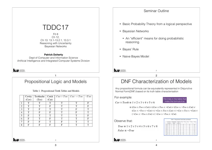
Seminar Outline • Basic Probability Theory from a logical perspective TDDC17 • Bayesian Networks Fö 8 Ch 12, • An “efficient” means for doing probabilistic Ch 13: 13.1-13.2.1, 13.3.1 reasoning. Reasoning with Uncertainty Bayesian Networks • Bayes’ Rule Patrick Doherty • Naive Bayes Model Dept of Computer and Information Science Artificial Intelligence and Integrated Computer Systems Division 2 1 2 DNF Characterization of Models Propositional Logic and Models Any propositional formula can be equivalently represented in Disjunctive Normal Form(DNF) based on its truth table characterisation For example: The lines in the table that make the formula true Cav ∨ Tooth ≡ 1 ∨ 2 ∨ 3 ∨ 4 ∨ 5 ∨ 6 ≡ ( Cav ∧ Too ∧ Cat ) ∨ ( Cav ∧ Too ∧ ¬ Cat ) ∨ ( Cav ∧ ¬ Too ∧ Cat ) ∨ ( Cav ∧ ¬ Too ∧ ¬ Cat ) ∨ (¬ Cav ∧ Too ∧ Cat ) ∨ (¬ Cav ∧ Too ∧ ¬ Cat ) ∨ (¬ Cav ∧ ¬ Too ∧ Cat ) ∨ (¬ Cav ∧ ¬ Too ∧ ¬ Cat ) Observe that: True ≡ 1 ∨ 2 ∨ 3 ∨ 4 ∨ 5 ∨ 6 ∨ 7 ∨ 8 False ≡ ¬ True 3 4 3 4

Degrees of Truth/Belief A Language of Probability • Truth Table Method: • Can be used to evaluate the Truth or Falsity of a formula • Just as propositional atoms provide the primitive vocabulary for propositions in propositional logic, random variables will provide the primitive vocabulary for our probabilistic language. 2 n n • Requires a table with rows, where is the number of propositional variables in the language • Random variables: • Propositional logic: • Allows the representation of propositions about the world which are True or False • Boolean: Cavity : { true , false } • In this case, a proposition has a degree of truth, either true or false • Discrete: Weather : { sunny , rainy , cloudy , snow } • Suppose our knowledge about the truth or falsity of a proposition is uncertain • Continuous: Temperature : { x ∣ − 43.0 ≤ x ≤ 100.0} • In this case we might want to attach a degree of belief in the propositions truth status • A random variable may be viewed as an aspect/feature of the world that is initially unknown • Observe that the degree of belief is subjective, in the sense that • A degree of belief may be attached to a variable/value pair • the proposition in question is still considered to be true or false about the world • We simply do not have enough information to determine this. • Complex formulas may be formed using Boolean combinations of variable/value pairs • So, there is a distinction between degrees of truth and degrees of belief Beliefs about Propositions Probability Degree of Belief Theory Propositional Propositions Degree of Truth Logic World 5 6 5 6 Probability Distributions Joint Probability Distributions Assume a domain of random variables: { X 1 , …, X n } P ( Weather = sunny ) = 0.7 P ( Cavity = true ) = P ( cavity ) = 0.4 P ( Weather = rainy ) = 0.2 P ( Cavity = false ) = P (¬ cavity ) = 0.6 P ( X 1 , …, X n ) A full joint probability distribution , assigns a probability to each of the possible combinations of variable/value P ( Cavity ) = ⟨ 0.4,0.6 ⟩ P ( Weather = cloudy ) = 0.08 pairs P ( Weather = snow ) = 0.02 P ( Cavity , Weather ) = ⟨ 0.30,0.05,0.145,0.005,0.30,0.05,0.145,0.005 ⟩ (2 x 4) P Notation P ( Weather ) = ⟨ 0.7,0.2,0.08,0.02 ⟩ P notation: can also mix variables and specific values: P ( X ) is the Probability Distribution (Unconditional or Prior P ( cavity , Weather ) = ⟨ 0.35,0.05,0.145,0.005 ⟩ (1 x 4) X Probability of the random variable P ( Cavity , Weather = rainy ) = ⟨ 0.1,0.1 ⟩ (2 x 1) 7 8 7 8

An Example Using a Full Joint Probability Distribution Using a full joint probability distribution, arbitrary Boolean combinations of variable value pairs can be interpreted by taking the sum of the beliefs attached to each interpretation (atomic event) which satisfies the formula. Each logical model is Recall our DNF characterisation an atomic event of logical formulas! P ( cav ∨ too ) = 0.108 + 0.012 + 0.072 + 0.008 + 0.016 + 0.064 = 0.28 P ( cav → too ) = 0.108 + 0.012 + 0.016 + 0.064 + 0.144 + 0.576 = 0.2 P (¬ too ) = 0.072 + 0.008 + 0.144 + 0.576 = 0.8 P (¬ too ) = 1 − P ( too ) = 1 − (0.108 + 0.012 + 0.016 + 0.064) = 0.8 9 10 9 10 Conditional Probability P Some additional notation In classical logic, our main focus is often: Γ ⊧ α P ( X ∣ Y ) P ( X = x i ∣ Y = y j ) i j denotes the set of equations for each possible , . In probability theory, our main focus is often: P ( X ∣ Y ) For example: P ( X ∧ Y ) = P ( X , Y ) = P ( X ∣ Y ) * P ( Y ) Prior probabilities are not adequate once additional evidence concerning previously unknown random variables is introduced: • One must condition any random variable(s) of interest relative to the new evidence. • Conditioning is represented using conditional or posterior probabilities. P ( X = x 1 ∧ Y = y 1 ) = P ( X = x 1 ∣ Y = y 1 ) * P ( Y = y 1 ) P ( X = x 1 ∧ Y = y 2 ) = P ( X = x 1 ∣ Y = y 2 ) * P ( Y = y 2 ) X = x i Y = y j P ( X = x i ∣ Y = y j ) The probability of given is denoted ⋮ P ( X = x i ∧ Y = y j ) = P ( X = x i ∣ Y = y j ) * P ( Y = y j ) P ( X = x i ∧ Y = y j ) P ( X = x i ∣ Y = y j ) = P ( Y = y j ) Note also that: P ( X ∧ Y ) = P ( X , Y ) Conjunction is abbreviated as a “,” Another way to write this is in the form of the product rule: P ( X = x i ∧ Y = y j ) = P ( X = x i ∣ Y = y j ) * P ( Y = y j ) P ( X , Y ) is also a distribution so it is equal to a vector This rule can be generalised if we have the distribution giving the chain rule P ( X = x i ∧ Y = y j ) = P ( Y = y j ∣ X = x i ) * P ( X = x i ) 11 12 11 12

Kolmogorov’s Axioms Some Useful Properties In probability theory, the set of all possible worlds is called the Δ Recall our discussions about logical theories, , consisting Ω sample space, . Let ω refer to elements of the sample space Δ ⊧ α of a set of axioms and our interest in Ω (models/interpretations). Assume is a discrete countable set of worlds. Probability Theory can be built up from three axioms: 0 ≤ P ( ω ) ≤ 1 ω , for all . 0 1 1. All probabilities are between and . a 0 ≤ P ( a ) ≤ 1 • For any proposition , . ∑ P ( ω ) = 1 P ( True ) = 1 2. Necessarily true (i.e. valid) propositions have 1 probability , and necessarily false propositions ω ∈Ω 0 have probability . P ( True ) = 1 P ( False ) = 0 ϕ P ( ϕ ) = ∑ and . • P ( ω ) For any proposition , 3. The probability of a disjunction is given by: P ( a ∨ b ) = P ( a ) + P ( b ) − P ( a ∧ b ) ω ∈ ϕ • 13 14 13 14 Some Examples Marginal Probability & Marginalization P ( Y ) = ∑ P ( Toothache , Cavity , Catch ) P ( Y , z ) Joint probability distribution : Marginal probability of Cavity ∧ Catch z Y = { Cavity , Catch } Z = { Toothache } Let and P ( Y ) = P ( Y , toothache ) + P ( Y , ¬ toothache ) 0.2 P ( cavity , catch ) = P ( cavity , catch , toothache ) + P ( cavity , catch , ¬ toothache ) Marginalization is about extracting the distribution over = 0.108 + 0.072 = 0.18 some subset of variables or a single variable Marginal probability of Cavity The marginal probability of Cavity is: Y = { Cavity } Z = { Catch , Toothache } Let and P ( Cavity ) = 0.108 + 0.012 + 0.072 + 0.008 = 0.2 P ( Y ) = P ( Y , catch , toothache ) + P ( Y , ¬ catch , toothache )+ ∑ P ( Y , catch , ¬ toothache ) + P ( Y , ¬ catch , ¬ toothache ) Y Z Let and be sets of variables, and where sums over all possible combinations z Z P ( cavity ) = P ( cavity , catch , toothache ) + P ( cavity , ¬ catch , toothache )+ of values of the set of variables . Then the general marginalization rule is: P ( Y ) = ∑ P ( cavity , catch , ¬ toothache ) + P ( cavity , ¬ catch , ¬ toothache ) P ( Y , z ) = 0.108 + 0.012 + 0.0720.008 = 0.2 z 15 16 15 16